|
|
Figure and Table Captions
|
 |
Figure
1. Narrow-Azimuth Design A. The recording patch is 10 lines of 96
channels with individual channels spaced 220 feet apart.
The
receiver lines are 880 feet apart. Overall, the resulting
rectangular geometry is 20,900 feet long in the in-line direction
and 7920 feet wide in the cross-line direction. |
|
 |
Figure
2. Wide-Azimuth Design B. The recording patch is 10 lines of 96
channels with individual channels spaced 220 feet apart.
The
receiver lines are 2200 feet apart. Overall, the resulting square
patch is 20,900 feet long in the in-line direction and 19,800 feet
wide in the cross-line direction. |
|
 |
Figure
3. Wide-Azimuth Designs C and D. The recording patch is 24 lines of
96 channels with individual channels spaced 220 feet apart.
The
receiver lines are 880 feet apart. Overall, the resulting square
patch is 20,900 feet long in the in-line direction and 20,240 feet
wide in the cross-line direction. |
|
 |
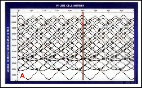
Figure
4A. "Necklace" plot for Narrow-Azimuth Design A. For these displays
the Y (vertical) axis indicates source-to-detector offset distance
in feet for each pre-stack trace within a cell. The X (horizontal)
axis shows subsurface cell location. In-line cell number 140 has
been highlighted to show all trace offset distances for a single
cell. The offset distribution for this design is fairly uniform with
30 individual offset traces between 0 and 11,000 feet at cell number
140, for example. This should produce better results during data
processing. |
|
 |
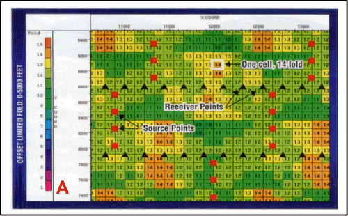
Figure 5A.
Offset-limited fold plot for Narrow-Azimuth Design A. Figures 5A,
5B, 5C, and 5D show a magnified portion of the fold plot that
results when source-to-detector offsets are limited to 0 to 5000
feet. Individual cells or subsurface bins are delineated as squares.
Trace count in any given cell is indicated by both the color
and
number within each square. Offset-limited fold for this design is
much higher than designs B or C, and ranges from 10 to 14. |
|
 |
Figure
4B. "Necklace" plot for Wide-Azimuth Design B. This design will
produce large gaps in offset domain sampling of the data, where from
0 to 4000 feet there are only two offset traces. |
|
 |
Figure
5B. Offset-limited fold plot for Wide-Azimuth Design B. Offset
limited fold for design B is from 4 to 7 fold. |
|
 |
Figure
4C. "Necklace" plot for Wide-Azimuth Design C. As with design B,
this design will result in very irregular sampling of
source-to-detector offset distances, where from 0 to 4000 feet there
are only three offset traces. |
|
 |
Figure
5C. Offset-limited fold plot for Wide-Azimuth Design C. Offset
restricted fold for design C fold is similar to design B. It ranges
from 4 to 8 fold. |
|
 |
Figure
4D. "Necklace" plot for Wide-Azimuth Design D. Design D has better
offset sampling than the other three designs, but it is also much
higher fold. It has 72 individual offset traces between 0 and 11,000
feet. |
|
 |
Figure
5D. Offset-limited fold plot for Wide-Azimuth Design D. The offset
limited fold for design D (10 to15) is only slightly higher than
Narrow-Azimuth Design A despite having nominal fold that is more
than twice as high. Most of the extra fold consists of longer
offsets in the cross-line direction.
Click to view comparison of necklace plots
for narrow-azimuth design A (Figure 4A) and for wide-azimuth designs
B, C, and D (Figures 4B, 4C, and 4D).
Click to view comparison of offset-limited
fold plots for narrow-azimuth design A (Figure 5A) and for
offset-limited fold plots for wide-azimuth designs B, C, and D
(Figures 5B, 5C, and 5D). |
|
 |
|
|
 |
|
Return to top.
There is
no short and simple answer to the question of optimum source-to-detector
azimuth. Intuitively, a wide-azimuth survey that collects long offset
data from all directions might seem to be better -- but this is not
always the case. In fact, most early  3-D 3-D seismic surveys were narrow
azimuth, although it was probably a matter of necessity as much as
intentional design. In basins with moderate-to-deep objectives, the
number of channels in the recording system restricted the contractors'
ability economically to acquire wide-azimuth seismic data. seismic surveys were narrow
azimuth, although it was probably a matter of necessity as much as
intentional design. In basins with moderate-to-deep objectives, the
number of channels in the recording system restricted the contractors'
ability economically to acquire wide-azimuth seismic data.
However,
most of these early surveys were "good enough" to be considered
successful, or if they were not, it probably was not the lack of azimuth
that caused them to fail. For deep geologic objectives, equipment
limitations can still exist. Achieving long offsets in the cross-line
direction requires either very widely spaced receiver lines or a lot of
lines in the active recording patch.
Before choosing a wide-azimuth design, a
question that must be asked is how will these different azimuths be
used? If pre-stack, azimuthally dependent analysis of the data is
planned (see, for example, Search and
Discovery Article #40098 (2003), “3-D
Seismic Data in Imaging Fracture Properties for Reservoir Development,”
by Bob Parney and Paul LaPointe),
then wide-azimuth data is absolutely necessary. If not, designing
a survey to record long offsets in all directions can easily create more
problems than it solves.
To help
understand the implications of wide-azimuth shooting, comparison is made
of offset-distribution plots from a standard narrow-azimuth geometry
(Figure 1, Design A) to three different wide-azimuth designs (B, C, and
D). However, before doing that, a careful look at each of the four
different acquisition strategies should be made.
For all
four surveys we will assume a maximum usable offset of 10-11,000 feet.
Other key design parameters are listed in Tables
1 and 2. In particular,
notice the "Maximum Cross-Line Offset" values listed in
Table 2. As
shown in Figure 2, wide-azimuth design B has greater cross-line offset
than narrow-azimuth design A (Figure 1), despite having the same number
of receiver lines, channels, and fold. It does this by using a receiver
line spacing that is more than twice the spacing used for design A.
Design C
(Figure 3), on the other hand, has the same receiver line spacing as A
(the narrow design), but uses 24 lines in its patch geometry to achieve
the added width. However, to keep the fold (and cost) about the same as
that of the narrow design, source line spacing for C has more than
doubled.
Finally,
there is design D -- the "best" of the wide designs. It uses the same
source and receiver line spacing as the narrow plan. The major design
difference is in its recording patch -- 24 lines of 96 channels versus
only 10 lines for A. As a result, the fold produced by design D will be
more than twice that of the other surveys. There is one other difference
between these two designs: relative cost. Design D will cost more to
acquire, because significantly more recording equipment will be needed.
For any
particular 3-D survey design, a wide range of attribute plots can be
easily produced and examined. However, for any given fold, the attribute
that will have the most impact on data quality is offset distribution.
The potential problems created by poor (irregular) offset distribution
are numerous, and in some cases the damage is irreparable by even the
cleverest data processor.
These
problems might include (but limited to) the following processing related
issues:
-
DMO (Dip Move Out)
artifacts.
-
Poorly resolved
surface-consistent statics solutions.
-
Poorly resolved refraction
statics solutions.
-
Inferior, or highly
variable stack attenuation of coherent noise.
-
Degraded AVO analyses.
-
Increased appearance of an
acquisition footprint.
-
Increased difficulty
estimating correct processing velocities.
-
Certainly,
not all surveys with poor offset distribution will be ruined by problems
such as these, but it is better to address them during the design phase
than after the data are acquired. We shall examine offset distribution
plots and offset-limited fold plots from several different wide-azimuth
designs. We shall also compare these plots to similar plots from a
typical narrow-azimuth design. This comparison will reveal some of the
adverse effects that can result from wide-azimuth shooting.
Given the
importance of source-to-detector offset distribution for each individual
cell, for any given fold and bin size, offset distribution is the single
most important design attribute, especially when it comes to processing
and interpreting the final data volume.
One of the
best ways to display this offset information is with a trace offset
scatter plot -- also known as a "necklace plot," which displays
source-to-detector offset distances (along the vertical axis) for every
pre-stack trace that belongs within a particular cell. Adjacent cells
are indicated along the horizontal axis, so that entire cell-lines can
be examined at one time. Gaps in offset-domain coverage appear as voids
in a pattern of overlapping "necklaces." The larger the void is, the
greater the likelihood of noticeable artifacts in the processed data.
Figures 4A
and 4B are necklace plots that correspond to designs A and B (Figures 1
and 2). Recall that design A is the narrow-azimuth survey, where the
cross-line maximum offset is only about 40 percent of the in-line
maximum. Design B, on the other hand, has in-line and cross-line maximum
offsets that are approximately equal to each other.
Note that
even though designs A and B produce the same fold, the offset
distribution for the wide design (Figure 1B) is markedly poorer. The
same observation also holds true for Wide Azimuth Design C (Figure 4C).
In both cases, near and mid-range offsets have been sacrificed in order
to achieve large cross-line offsets. As a result, the data volume
produced by either design B or design C is likely to be inferior to the
volume produced from A -- the narrow design.
Of the
three wide-azimuth designs modeled, only design D has better offset
distribution (Figure 4D) than design A. However, the D design also has
more than two and a half times the fold of A, and that extra fold does
not come free. The cost of acquiring design D will be substantially
higher than any of the other three designs.
In
addition to having poor offset distribution, the ability of designs B
and C to image shallow events is degraded. We can see this degradation
by examining fold plots that have been offset-limited to
source-to-detector distances of 5000 feet or less (Figures
5A, 5B,
5C,
and 5D). Limiting the offsets to 5000 feet or less is representative of
the offset mute that is applied to shallow data by the data processors.
For this
example, we will consider geologic depths of about 4000 to 6000 feet to
be "shallow." Although the nominal fold for Wide-Azimuth Designs B and C
is about the same as Narrow-Azimuth Design A, the offset-restricted fold
is quite different. Figure 5A shows that offset-restricted fold for
design A ranges from 10 to 14, whereas the wide designs B and C (Figures
5B and 5C) only have four to eight traces per cell. This means the
ability to map a shallow, secondary objective accurately, or to use a
shallow marker horizon for isochron mapping, probably will be
compromised by using either design B or C. Only design D achieves
wide-azimuth data and effective imaging of shallow events (Figure 5D).
Unfortunately, as we have noted before, design D will cost more to
acquire than any of the other three design options.
The
specific point of this article is not to suggest that designs B, C or D
are necessarily better -- or worse -- than design A. Rather, it is to
call attention to the fact that those extra azimuths are going to cost
you in one way or another. Either the price of your seismic survey will
go up, or the offset distribution and shallow imaging will deteriorate,
or both. Therefore, you must carefully weigh the pluses against the
minuses in the final seismic subsurface image. What are you getting?
What are you losing? What will it cost?
Overall,
the best overall 3-D seismic survey is not necessarily the one with the
best quality data; nor does it have to be the one with long offset data
from all azimuths. The best survey really depends on balancing a
combination of factors -- in particular, subsurface geology and economic
objectives. For some projects, wide-azimuth data is a necessity; for
others, it can be more of a liability than an asset. The critical issue
is to record seismic data that are "good enough" to image the geology
and still meet the economic requirements of the user. This is
accomplished by recognizing the important role of survey design in the
planning process. seismic survey is not necessarily the one with the
best quality data; nor does it have to be the one with long offset data
from all azimuths. The best survey really depends on balancing a
combination of factors -- in particular, subsurface geology and economic
objectives. For some projects, wide-azimuth data is a necessity; for
others, it can be more of a liability than an asset. The critical issue
is to record seismic data that are "good enough" to image the geology
and still meet the economic requirements of the user. This is
accomplished by recognizing the important role of survey design in the
planning process.
Acknowledgments
Dan
Wisecup and Kevin Werth assisted in the preparation of this article.
Figures 1-3 are courtesy of Kevin Werth.
Return to top.
|