GCAutotracking Horizons in ![]() Seismic
Seismic![]() Records*
Records*
Satinder Chopra¹ and Kurt J. Marfurt²
Search and Discovery Article #41489 (2014)
Posted November 17, 2014
*Adapted from the Geophysical Corner column, prepared by the authors, in AAPG Explorer, November, 2014, and entitled "Autotracking Your Way to Success". Editor of Geophysical Corner is Satinder Chopra ([email protected]). Managing Editor of AAPG Explorer is Vern Stefanic.
¹Arcis ![]() Seismic
Seismic![]() Solutions, TGS, Calgary, Canada ([email protected])
Solutions, TGS, Calgary, Canada ([email protected])
²University of Oklahoma, Norman, Oklahoma
A horizon is a reflection surface picked on a 3-D ![]() seismic
seismic![]() data volume that is considered to represent either a lithologic interface or a sequence stratigraphic boundary in the subsurface. Usually, an interpreter begins the exercise of identifying the different subsurface horizons by correlating the available well log data with the
data volume that is considered to represent either a lithologic interface or a sequence stratigraphic boundary in the subsurface. Usually, an interpreter begins the exercise of identifying the different subsurface horizons by correlating the available well log data with the ![]() seismic
seismic![]() data. In its simplest form, such identification can be done by hanging an impedance log curve on the
data. In its simplest form, such identification can be done by hanging an impedance log curve on the ![]() seismic
seismic![]() data – or more quantitatively, by generating a synthetic seismogram from the impedance log curve using an appropriate wavelet and correlating the result with measured
data – or more quantitatively, by generating a synthetic seismogram from the impedance log curve using an appropriate wavelet and correlating the result with measured ![]() seismic
seismic![]() traces about the well. Depending on the
traces about the well. Depending on the ![]() seismic
seismic![]() data quality and either the presence or lack of isolated strong reflectors, identifying horizons can be a trivial exercise or a challenging problem.
data quality and either the presence or lack of isolated strong reflectors, identifying horizons can be a trivial exercise or a challenging problem.
|
♦General statement ♦Figures ♦Metod ♦Examples ♦Conclusions
♦General statement ♦Figures ♦Metod ♦Examples ♦Conclusions
♦General statement ♦Figures ♦Metod ♦Examples ♦Conclusions
♦General statement ♦Figures ♦Metod ♦Examples ♦Conclusions
♦General statement ♦Figures ♦Metod ♦Examples ♦Conclusions
♦General statement ♦Figures ♦Metod ♦Examples ♦Conclusions |
In the beginning, horizons were handpicked, posted on a map and hand-contoured. In the 1970s and 1980s the hand picks were manually digitized by a technician, loaded into a database and then contoured using a mainframe computer. Removing bad picks from the database required extra requests. Such a task was laborious, inefficient and usually not very accurate. With the introduction of the workstations, this task became automated – much to the relief of the Today's automated horizon-picking algorithms are much more sophisticated than those of a decade ago. While automated pickers appear to simply find peaks, troughs and zero-crossings on adjacent traces, internally there are constraints of correlation coefficient, dip and coherence that provide the ability to pick through moderate quality data with relatively complicated waveforms. Nevertheless, autotracking is sensitive to the variations in the signal-to-noise (S/N) ratio of the
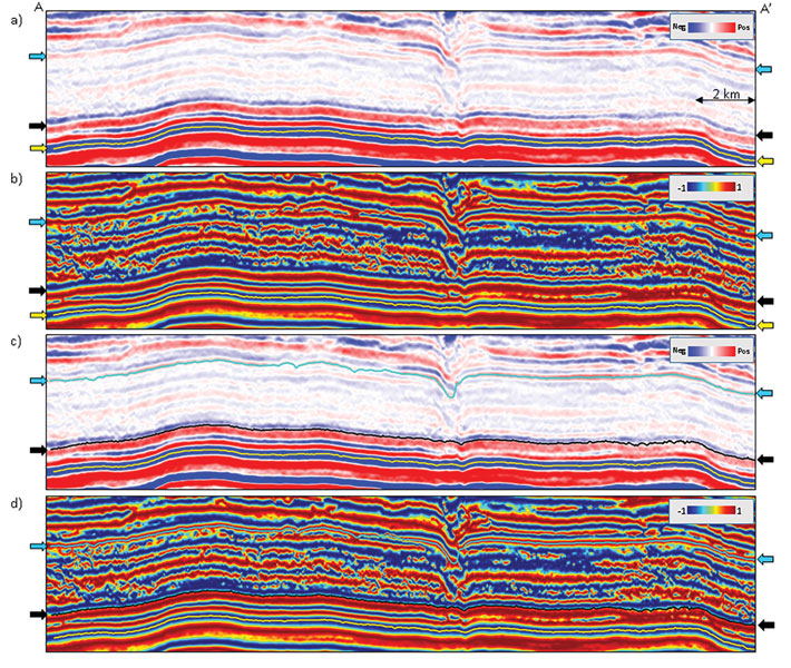
Autotracking works very well on coherent Because of lateral changes in overburden and A question that usually arises is: Why should one pick a zero-crossing if the If the objective is to map a thin bed, the well tie is usually a zero-crossing. Our experience has shown that In Figure 1 we show a In Figure 2, we show the equivalent segment of the The take-away from this simple exercise is that horizons could be picked along zero-crossings in preference to peaks or troughs. If the well tie is to a peak or trough, one simply computes the quadrature (also called the Hilbert transform and the imaginary part) of the Not all geological markers of interest may correspond to a strong peak or a strong trough. Many times a horizon has to be tracked along a weak amplitude peak or trough, where autotracking breaks down. In such cases the use of In the November 2004 Geophysical Corner – Search and Discovery Article #40141, an interesting application in terms of the use of the cosine of instantaneous phase attribute for autotracking was discussed. The complex trace attributes serve to examine the amplitude, phase and frequency delinked from each other. The instantaneous phase attribute can be analyzed without the amplitude information, but is discontinuous for both 180 degrees and -180 degrees. The cosine of instantaneous phase has a value of unity for both these angles, and so is a better attribute to pick horizons on. In Figure 3a we show a segment of a The equivalent cosine of instantaneous phase attribute section is shown in Figure 3b. Horizons are tracked corresponding to the zero-crossings along the blue and black arrows on this data volume (Figure 3d) and overlaid on the In Figure 4a we show the display of the autotracked horizon attempted on the Most autotrackers internally use a cross-correlation algorithm to compare adjacent waveforms. Weak reflectors can be overpowered by adjacent stronger reflectors as well as by stronger cross-cutting noise. By balancing the amplitude, the cosine of instantaneous phase attribute minimizes these interference effects. If horizons are autotracked along zero-crossings on 3-D |