![]() Click to view article in PDF format.
Click to view article in PDF format.
A Petrophysical Method to Evaluate Irregularly Gas Saturated Tight Sands Which Have Variable Matrix Properties and Uncertain Water Salinities*
Michael Holmes1, Dominic Holmes1, and Antony Holmes1
Search and Discovery Article #40673 (2011)
Posted January 11, 2011
*Adapted from oral presentation at AAPG International Conference and Exhibition, Calgary, Alberta, Canada, September 12-15, 2010
1Digital Formation, Denver, Colorado ([email protected])
A problem in many Rocky Mountain tight gas sandstones is a sequence that is only partially gas saturated, with changing matrix properties combined with variable (and often unpredictable) water salinities. Often it is difficult to distinguish between high resistivity fresh water wet sands, and high resistivity, gas-bearing sands. A standard approach is to make a qualitative judgment based on density/neutron response – the gas “cross-over” effect. However, if matrix properties are variable, this approach can be misleading, and is at best a qualitative judgment.
The methodology presented here is a quantitative assessment of gas saturation by comparing matrix specific density and neutron responses with porosity, calculated such that gas effects are minimized. Cross plot porosity from density/neutron combination is only minimally affected by gas and by changing matrix properties.
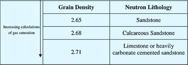
Three sets of calculations are made assuming sandstone (bulk density 2.65 gm/cc), calcareous sandstone (bulk density 2.68 gm/cc) and heavily cemented calcareous sandstone, or limestone (bulk density 2.71 gm/cc). Quantified estimates of gas saturation, as “seen” by each log, are available for each assumed rock type. Pressure effects on porosity log responses are included in the calculations.
Four sets of saturation profiles are now available, one from standard resistivity log analysis and three from porosity log analysis assuming different matrix properties. Comparisons among the 4 sets of saturation profiles can be combined with other data, such as mud log shows and (if available) core measured matrix densities. Using such comparisons, it is often relatively simple to distinguish between wet intervals and gas-bearing intervals. With increasing assumed grain density, gas saturations calculated from the porosity logs increase. If gas saturations so defined are unrealistically high, it is an indication that actual grain density is less than assumed grain density.
Additionally, if matrix properties are well-defined, it is possible to verify Rw input for resistivity log interpretation, and adjust as necessary. It is important to recognize that the porosity logs, and particularly the density log, investigate close to the wellbore, and may well be influenced entirely by the flushed zone. Examples are presented from Rocky Mountain reservoirs, in sequences where the problem of irregular gas saturation in systems with variable Rw is particularly severe.
Copyright � AAPG. Serial rights given by author. For all other rights contact author directly.
|
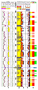
Shaley Formation Resistivity Analysis
The interpretation is a standard shaley formation analysis, involving calculations of total porosity, shale volume, and total water saturation. One of the issues in tight gas sands is the correct choice of matrix lithology. If only a density log is used, the correct choice of grain density is crucial. In the event of lack of core data this may be particularly problematic, especially if grain density is variable. By using a density/neutron cross plot, this restriction is overcome. Fluid density is a required input, and should be estimated from a reasonable assumption of gas saturation close to the wellbore. A porosity/resistivity cross plot can help in this choice.
The second set of analysis involves the calculation of effective porosity and water saturation (i.e. removing the effects of clay). From these calculations, again based on resistivity interpretations, potential mobile water and/or poor quality reservoir rock can be distinguished from capillary bound water. Lack of light blue color fill on Figure 2, track 4 and Figure 4, track 3 equates to better quality, gas-bearing reservoirs. Example of application of these techniques are described in AAPG Annual Convention, June 2009 “Relationship Between Porosity and Water Saturation: Methodology to Distinguish Mobile from Capillary Bound Water ” by Michael Holmes, Antony Holmes, Dominic Holmes.
Gas Saturation from Porosity Logs
Comparison of density with neutron logs is used routinely for a qualitative assessment of the presence of gas – the density/neutron “cross-over” effect. The response is controlled by the concentration of hydrogen in the pore space. Because gas contains less hydrogen than oil or water, apparent neutron porosity is suppressed. The cross plot (Figure 1) shows the effects of gas. Porosity values are lithology specific, i.e. raw logging data must be converted to a known (or presumed) lithology. By assuming different lithologies, the cross plot can be solved for gas saturation. The assumption is made that the density and neutron logs both investigate about the same volume of rock – or, as in the case of tight gas sands, there is a little variation of gas saturation away from the wellbore (minimal or no invasion by drilling fluid). Three different lithologies are assumed in this paper:
Standard resistivity interpretation from a Piceance Basin well, NW Colorado, is shown in Figure 2. Interpretation of the porosity resistivity cross plot (Figure 3) shows input used for saturation determination:
Rw = 0.1 Water resistivity a = 1.0 Cementation constant m = 2.0 Cementation exponent n = 1.7 Saturation exponent
A summary of the interpretation is as follows:
Figure 4 shows the same interval as Figure 2, with the addition of interpretations of gas saturation from porosity logs. Examination of the porosity log Sg data shows the following:
|