Introduction
We provide a rationale for rapidly assessing the depth and structure of sedimentary basins from magnetic anomaly data. Our methodology is based on Tilt-Depth calculated strictly from first-order derivatives of the total magnetic field. We assume a simple buried vertical contact model such as the 0 degree contour of the Tilt derivative of RTP magnetic data closely follows the edge of the vertical contact, while the distance between the ±45° contours provides an estimate of the depth to the top of the buried contact. We have applied the Tilt-Depth method to magnetic data covering various sedimentary basins within the African continent.
Magnetic Data for Basin Mapping
Magnetic data play a crucial role at various stages of hydrocarbon exploration, beginning with the definition of basins in frontier areas (Figure 1). Analysis of magnetic data using special techniques provide estimates of depth to basement. The Tilt-Depth method is a new technique to map variations in basement depth directly from magnetic maps.
Magnetic Derived Parameters:
1) Depth to magnetic basement
2) Strike of contacts/faults
3) Dip of contact
4) Susceptibility contrast
Tilt-Depth Method: Theory and Simple Examples
The Tilt-Depth method (Salem et al., 2007), based on a model of a buried 2D vertical contact, provides a relatively simple means to estimate location and strike of geological contacts/faults and depth to basement from RTP magnetic anomalies. The horizontal and vertical derivatives of the observed magnetic field are given by:
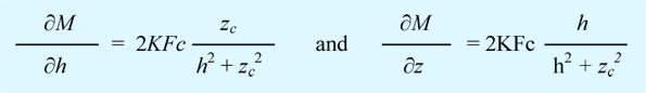
where h=0 and z are the horizontal and vertical locations of the contact respectively, k is susceptibility contrast and is the magnitude of the magnetic field. The parameter c is given by c=1-cos2i sin2A, where A is the angle between the positive h-axis and magnetic north, i is the ambient field inclination, tanl=tani/cosA, d is the dip (measured from the positive h-axis), and all trigonometric quantities are in degrees. Substituting the above derivative terms into the Tilt equation and assuming a Reduced-to-Pole field, it can be shown that
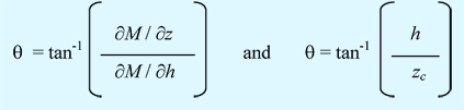
The Tilt equation indicates that the horizontal location of the contact (h=0) occurs where Tilt=0°, and h=±qzc when q=±45°, respectively. Thus, depth can be estimated directly from a map of the Tilt derivative by measuring the distance between appropriate contours, hence the name Tilt-Depth. Figure 2 shows the vertical 2D contact model and the resulting Tilt derivative profile for a geomagnetic inclination of 90. The section of the Tilt anomaly between the range 45 is shaded. The value of the Tilt angle above the contact is 0° (h=0), and is +45° when h=zc and -45° when h=-zc.
This suggests that contours of the magnetic Tilt angle can identify both the location and depth (half the physical distance between ±45° contours) of contact-like structures. Figure 3A shows the contoured RTP field over 3D model structures (outlined as colour polygons) at 4 km depth (NW body) with susceptibility 0.002 SI and at 8 km depth (SE body) with susceptibility of 0.001 SI. Figure 3B shows the Tilt anomaly calculated from the polygon anomalies, restricted to values lying between ±45°.
The colour fill between these contours represents the depth estimate which varies due to anomaly interference and non 2D structural affects. The examples shown utilize the 45° Tilt derivative contours;
other Tilt angles can be used with an appropriate factor to convert the distance between the contours to depth.
Application in Tanzania
In this section we demonstrate the Tilt-Depth method on aeromagnetic data over the Karoo sedimentary rift structures of southeast Tanzania. The regional geological setting is a consequence of the breakup of Gondwana and rifting along the eastern margin of Africa. The Selous Basin is a NNE-SSW trending rift basin infilled with up to ~10 km of mainly non-marine and non-magnetic sediments ranging in age from Permian-Triassic to Tertiary. The basin is bounded to the west and east by shallow basement with the Masasi Spur separating the Selous Basin from the coastal basins of eastern Tanzania. The Rufiji Trough is located to the northeast of the Selous Basin and exhibits E-W extensional structures of Jurassic age superimposed on earlier NNE-SSW trending structures.
A countrywide aeromagnetic grid for Tanzania has been compiled by GETECH from 1 km spaced flight-line data oriented predominantly E-W, with a mean terrain clearance of 120m. The resulting grid has a nodal separation of 0.25 km. Figure 4 shows the TMI anomaly map over the study area and clearly delineates the rift basin outline by the shape change in the frequency content of the magnetic anomalies. Before applying the Tilt-Depth method, the data were converted to RTP using a magnetic inclination of -40° and a declination of -3.5°, and upward continued to a distance of 1 km.
The Tilt-Depth map (Figure 5) defines regions of shallow basement (the Masasi Spur, and the region west of the Selous Basin), characterized by numerous closely-spaced lineaments, with corresponding depths shallower than 4 km. Within the Selous Basin and Rufiji Trough, the Tilt ±45° contours are much more widely spaced. These contours define magnetic lineaments within the basin, as well as areas of more chaotic contours which in part could be due to anomaly interference. Basement depths in the Selous Basin range from 3 to 6 km while in the Rufiji Trough they increase to 8 km. These depths show a good correspondence with the regional variation in sediment thicknesses based on seismic and well control data.
Interpolation of the Tilt-Depth results leads to an initial depth to basement map covering the entire basin area, Figure 6, along with other magnetic derivative maps (for example the Tilt derivative itself, Figure 7. These maps, should be viewed as stage products from which structure and depth maps can be constructed, Figure 8.
Reference
Salem, A., S. Williams, J. D. Fairhead, D. Ravat and R. Smith, 2007, Tilt-depth method; A simple depth estimation method using first-order magnetic derivatives: SEG The Leading Edge, v. 26/12, p. 1502-1505.
return to top |


