Click to view article in PDF format.
Rock Property Data Volumes from Well Logs*
By
L.R. Denham1 and H. Roice Nelson, Jr. 2
Search and Discovery Article #40268 (2007)
Posted November 3, 2007
*Adapted from extended abstract prepared for poster presentation at AAPG Annual Convention, Long Beach, California, April 1-4, 2007
1Interactive Interpretation & Training, Inc., Houston, TX ([email protected])
2Geokinetics Processing & Interpretation, Houston, TX
Geology is sampled densely by wells vertically, but sparsely and irregularly horizontally. A modern seismic survey has sparse samples vertically, but close and uniform sampling horizontally. Seismic data is more useful for regional trends, but does not convey petrophysics, and is difficult to relate to wells. Inverting seismic data to resemble well data is almost impossible. Can we make well data resemble seismic data, not just a single-trace, but a complete volume?
We reduced well vertical sample interval to 60 m, computing numerous petrophysical properties. Then we computed vertical arrays of values for each property on a regular grid, using the samples computed at each well location. Wells within a specified radius were used, weighted inversely with distance, and well samples over a limited depth range, weighted inversely with depth difference from the sample depth. The computed three-dimensional array was written to disk in SEG Y format, and loaded into a seismic interpretation system.
In the initial project we generated data volumes for shale and sand P-wave velocities and densities, sand percentage, and pressure (mud weight), for most of the Gulf of Mexico. These volumes showed regional trends within the basin. The method has some problems in areas of sparse well information, and does not account for major structural features.
Petrophysical data volumes generated from well information allow the geologist to integrate information from thousands of wells using standard interpretation systems. So far, the technique seems to be more suited to regional analysis rather than to prospect development.
|
|
One of exploration’s perennial problems is relating well-derived geological information to seismic data. An additional tool for this is now available: data volumes of rock properties in SEG Y format, generated from well logs. These volumes are compatible with all standard seismic-interpretation systems and can be used by the interpreter to constrain interpretation of seismic data by giving the probable properties of rocks in an undrilled prospect.
How The Volumes Are Generated The starting point for the rock-property volumes is the standard suite of well logs. The standard set of rock properties in a dominantly clastic sequence is derived from velocity, density, and resistivity logs. Properties computed using fluid replacement require measurements or assumptions about properties of the fluids, such as oil and gas density, water salinity, and gas-oil ratio. Temperatures are based on measurements made while logging, and formation pressures are estimated from drilling mud weights. A petrophysicist classifies the rocks penetrated by each well, separating intervals into water-filled sand, shale, and all other lithologies (salt, coal, limestone, hydrocarbon-filled sand, etc.). These last intervals are excluded from the analysis. Wells are then divided into uniform depth intervals, using an interval large enough to contain significant quantities of both shale and water-filled sand, but small enough to adequately describe systematic variations. If the chosen interval is too small, many of the intervals will contain only sand, or only shale. If the interval is too large, there may be significant differences in rock properties from top to bottom, due to the difference in compaction, and more depth samples will include rocks with widely varying depositional environments. For the Gulf of Mexico examples described here, the interval chosen is 200 ft (61 m). For each interval, the averages of the fundamental properties of sand and shale are computed, along with the amounts of sand and shale within the interval and the variation of each property within the interval (recorded as standard deviation). Additional rock properties can be computed from the fundamental properties using standard procedures such as the Greenberg-Castagna technique (Greenberg and Castagna, 1992) for computing shear-wave velocities, inverse Gassmann’s equation (Gassmann, 1951) for computing dry-rock properties, and Gassmann’s equation along with the dry-rock properties to compute the properties of hydrocarbon-filled sands (Hilterman et al., 1999, Hilterman, 1990; Hilterman et al., 1998).
Once the well database is constructed, the SEG Y data volumes can be generated. There are several points to consider carefully:
When these questions are answered, the volume is generated. The process follows these steps for each trace:
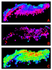
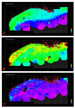
As each trace is completed, it is written in 32-bit floating point format to a standard SEG Y format file (Barry et al., 1975) which can be loaded into any seismic-interpretation system. The generation of these volumes takes time, so we generate graphical progress reports (updated every 1000 traces), allowing the user to check that the values used for interpolation and limits on the area covered are realistic without waiting for the job to finish. These plots are of two forms: maps (Figures 1, 2, 3a-c) and sections (Figure 3d).
The data volumes are loaded into standard seismic-interpretation systems (in this example, the Halliburton Landmark SeisWorks application), where they can be manipulated in the same way as ordinary seismic data. Figure 4a shows the P-wave velocity of water-filled sand in the western Gulf of Mexico (Texas to Alabama) at a depth 11,900 ft (3630 m) below the sea floor. The patches of background color left of the middle of the figure indicate areas where there is no well data available to this depth. The arcuate edges of data along the southern limits come from the distance limit on extrapolation from widely separated wells. Figure 4b shows a section through the same data volume, running from the middle of the Green Canyon area on the left to the Sabine Pass area on the right. The gaps in the bottom of the section mark areas with no deep wells (or no deep logs). The missing data at the top of the section at the left is where velocity logs were not available at depths less than 7500 ft (2290 m) below water bottom (the last 5% of the section depends on a single well). The white line marks the depth of geopressure as interpreted by examination of each well.
Uses for the Volumes These volumes have great potential for increasing an explorationist’s productivity and for defining more closely the risk of a prospect. Suppose, for example, you have identified a potential prospect on an OCS block in the Gulf, miles from the nearest existing well, and want to know whether the AVO anomaly associated with the prospect is what would be expected in that location at that depth, for either oil or gas. The usual solution is to model the AVO response. But the modeling program requires values for shale P-wave velocity (Figure 5a) and density (Figure 6b), sand P-wave velocity (Figure 3c, 4), sand density (Figure 1) and thickness, as well as depth (which can be determined from the seismic interpretation), mud weight (Figure 3), temperature (Figure 6a), gas density, oil density, gas-oil ratio, salinity and water saturation: a total of twelve unknowns. The new tool can provide a data volume derived from well data for six of those unknowns, so values can be extracted almost instantly. Only gas and oil density, gas-oil ratio, salinity, water saturation, and sand thickness remain, and hydrocarbon densities, gas-oil ratio, and salinity tend to vary relatively slowly from region to region. The interpreter can now concentrate on varying sand thickness and water saturation in the model, looking for a match to the observed AVO response. The variability of rock properties is important in estimating the probability of success for a prospect. Figure 6c shows the standard deviation of water-filled-sand velocities at 10,000 ft (3050 m) below the sea floor. This is one indicator of the variability of sand properties at this depth. Similar volumes can give actual measurements of the variability of other properties used for estimating probable reserves for a prospect. At a simpler level, the interpreter may need to know whether an observed change in amplitude at an apparent fluid contact is compatible with a change from water to oil. This question could be answered by comparing the difference in values from an oil sand reflectivity volume and a wet sand reflectivity model with the change in amplitude observed in the real seismic data in an intercept stack volume. This would be a deterministic solution analogous to the probabilistic solution described by Denham and Johnson (2006). On an even more basic level, a gross overview can be quickly accessed, with mud weight (Figures 3a and 3b), for example, showing regional variations in geopressure at any depth.
By combining two universally-used exploration tools – well logs as actual measurements of rock properties, and workstations for viewing three-dimensional data volumes – the explorationist can improve productivity and reduce risk by making better use of existing data. The missing link between the two tools is the uniformly-sampled data volume in a standard format, generated from irregularly-scattered well data.
Barry, K.M., Cavers, D.A., and Kneale, C.W., 1975, Report on recommended standards for digital tape formats: Geophysics, v. 40, no. 2, p. 344–352. Denham, L.R., and Johnson, D., 2006, Estimating probability of hydrocarbon content from seismic amplitude anomalies: Soc. Explor. Geoph. 76th Annual Meeting, INT3.3. Gassmann, F., 1951, Elastic waves through a packing of spheres: Geophysics, v. 16, no. 4, p. 673–685. Greenberg, M.L., and Castagna, J.P., 1992, Shear-wave velocity estimation in porous rocks: Theoretical formulation, preliminary verification and applications: Geophys. Prosp., v. 40, no. 2, p. 195–210. Hilterman, F., Sherwood, J.W.C., Schellhorn, R., Bankhead, B., and DeVault, B., 1998, Identification of lithology in the Gulf of Mexico: The Leading Edge, v. 17, no. 2, p. 215–222. Hilterman, F., Verm, R., Wilson, M., and Liang, L., 1999, Calibration of rock properties for deepwater seismic: 69th Ann. Internat. Mtg, p. 65–68. Hilterman, F., 1990, Is AVO the seismic signature of lithology? A case history of Ship Shoal-south addition: The Leading Edge, v. 9, no. 6, p. 15–22.
|