The Multiple Bischke Plot Analysis: A Simple and Powerful Graphic Tool for Integrated Stratigraphic Studies*
By
J-Y. Chatellier1 and C. Porras2
Search and Discovery Article #40110 (2004)
*Adapted from a poster-session presentation at the 2001 AAPG Annual Convention, Denver, Colorado, June, 2001, together with a revision presented at the 2003 CSPG Annual convention. The individual posters in PDF format may be viewed separately.
1PDVSA Oriente, Estudios Integrados Pirital, Puerto La Cruz, Venezuela; present address: Tecto Sedi Integrated, 271 Arbour Lake Way NW, Calgary, T3G 3Z7 Canada (email: [email protected])
2PDVSA Oriente, Estudios Integrados Pirital, Puerto La Cruz, Venezuela
Abstract
Establishing the correct stratigraphy is not always a simple task, especially when dealing with tectonically complex areas or where tectonics had locally controlled the sedimentation. Bischke (1994) introduced a simple technique to compare the gradual change in thicknesses in two wells, the difference being plotted against the reference well’s depth. The MBPA (Multiple Bischke Plot Analysis), derived from the original method, allows a very quick and objective review of the stratigraphy, whether it is done conventionally or using sequence stratigraphy.
The MBPA invokes many wells at the same time; thus, the problem well and the problem zone can be readily identified as the anomaly shows-up in all paired well comparisons. One of the interests of the method is that it does not matter how many faults or folds are present between the wells under study, as only disturbance within the wells will show-up in the analysis.
Stacking several Bischke plots on the same diagram gives a different view of the coherency of the stratigraphy and of the structure. Thus, trend-similarity is more obvious than in the MBPA, whereas local anomalies are less readily apparent.
The power and limitations of both methods are demonstrated through a review of case examples from various parts of the world. Thus, the MBPA allows one to quickly identify anomalies and to distinguish between faults of various types, unconformity, or wrong correlation. The method does not solve the problem but allows geoscientists to focus their attention on the real problem, be it a marker, a well, or a geographic area.
Complex sedimentology and active tectonism can be seen in a different way through the MBPA, especially when displaying the various Bischke plots on a map.
|
|
Bischke Plots
The original method was first published by Bischke in 1994 as the D/d plot. It was geared at understanding growth sedimentation patterns. A Bischke Plot allows you to check quickly and efficiently your correlation. The example in Figure 1.1 shows very well that the Bischke Plot gives full support to the interpreted faults in well 422, with well 593 supposedly being unfaulted. Faulted tops as well as drag folds are readily identifiable. Other faults of lesser magnitude could be proposed but would need extra support.
Brief Review of MBPA HistoryThe Multiple Bischke Plot Analysis (MBPA) (Figure 1.2) was devised by the first author in 1996 while revising the stratigraphy of the Furrial Field in Venezuela. The philosophy of the MBPA was summarized in Sanchez et al. (1997), whereas one case study from Lake Maracaibo was published in Chatellier et al. (1999). The present paper aims at stating our understanding of the power and limitation of the method that is becoming every day more popular, especially since the 1999 paper by Bischke et al.
A Bischke Plot: How Does It Work?--Graphical Explanation of the Method A "Bischke Plot," also called Dd/d diagram, is a graphical display of differences in depth of the various markers found in two wells (Y axis), plotted against the depth of the same markers in the reference well (X axis); all depths being true vertical depths (TVD). Alignment of points in a Bischke Plot indicates that the markers involved belong to series of rock with a similar and regular sedimentation pattern. The interest of the method is the opportunity given to graphically visualize existing breaks in the pattern. An apparent break in trend in a Bischke Plot can be attributed to many factors; these include:
All of these are possible in either well 1 or well 2 (Figures 2.1, 2.2, 2.3, and 2.4). A single Bischke Plot does not indicate in which well the problem lies. Note that changes in dip associated with fault drag alter the graphical relationship between markers and add hardship to the analysis. Stratal dip alone will not be reflected in a Bischke Plot if it stays constant (Figure 2.1). Figure 2.1 also shows that faults not intersecting a well will have no direct influence on a Bischke Plot. If a well is sufficiently close to a fault, some of the dips may be accentuated near the fault; that will be seen in the plot because of a larger apparent thickness than in the other well. Figure 2.2 also shows that,where no fault is present in a well, the fault will have no influence on a Bischke Plot. Where a well is intersected by a normal fault, values of the faulted sections affected by the fault will show values that are anomalous in comparison to younger and older beds. In Figure 2.3, two groups of tops (three markers each) form two parallel trends, but one point (green point--marker 3) does not fit on either trend because it has a faulted top; thus the encountered top is just an apparent top. Some of the dips may be accentuated near the fault; as noted above that will be seen in a plot, as there will be a larger apparent thickness than in the other well. Where a fault affects a section that includes an unconformity (Figure 2.4), the marker defining the faulted interval in the well (point No. 2--pink) stands out from both neighboring trends. This is because the top has been faulted out and the top encountered is not the true top. The change in slope may be indicative of growth faulting.
Poster 3 Figures
Figures 3.1 and 3.2 illustrate the usefulness of a single Bischke Plot in the study of a fault bend fold. Comparison of three Bischke plots involving three wells allows one to attribute the various anomalies to the proper wells. The examples in Figure 3.3 are from a well studied field in an extensional setting in Southeast Asia. A Multiple Bischke Plot Analysis allows one to identify wells that present very similar patterns and that can be grouped in families. The example in Figure 3.4 shows wells chosen at random from the Santa Barbara Field, Venezuela. It is the first attempt at a detailed stratigraphy currently under revision. The MBPA is an ideal tool for such a revision, as problems are readily visible. A larger number of markers gives a more reliable picture.
Poster 4 Figures
Coherency of Various Interpretations Validated by the MBPAWithin a common zone of interest in selected wells from Santa Barbara Field, Venezuela, 12 markers were used for interpretation 1 (with conventional stratigraphy) and 18 markers were used for interpretation 2 (within the framework of sequence stratigraphy) (Figures 4.1, 4.2, and 4.3). More layers do not mean more reliable stratigraphy. Further, sequence stratigraphy does not automatically mean correctness. Another example of coherency of correlation, with use of a Bischke Plot, is shown in Figure 4.4, from Maracaibo, Venezuela. The MBPA allows one to analyze objectively the relative coherency of various interpretations. It is better to be approximately right than precisely wrong.
Poster 5 Figures
VLA-31 Case Study: Block 1 Lake Maracaibo
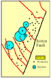
· Unsuccessful injection scheme. · Seismic indicates reverse faults. · Not a single repetition recognized in any of the wells.
Second step: Multiple Bischke Plot Analysis
Note that the red stratigraphic marker in Figure 5.3 is systematically an anomaly, whereas the blue stratigraphic marker is not anomalous in the comparison between well 753 and well 515. That part of the stratigraphic section is in the same block for both wells.
SolutionThe MBPA pin-pointed where the stratigraphic anomaly is in each well. The faults are sealing and oriented north-south. The strike-slip hypothesis explains why no repetition was seen in any of the reverse faults (Figure 5.4). The hypothetical fault planes confirmed the seismic interpretation (Figure 5.5).
Poster 6 Figures
Power and Limitation of the MBPA: Examples from the Western Canada Basin
MBPA in Very Complex Part of Western Canada BasinWhen the area under study is very complex, a map display of the various Bischke plots can be very useful. Thus the tectonic activity of the faults can be assessed in terms of timing and intensity. Figure 6.1 represents a “first glance” at a new area. The findings from MBPA have been corroborated by seismic. In Figure 6.1, maximum tectonic activity was at the time that the red marker was deposited. In the western part of the area, earlier tectonic activity is indicated by the green marker moving away from the trend expressed by the underlying units. The angle between the observed trends is indicative of how strong the tectonic activity was at the time represented by the red marker.
MBPA Expression of Clinoform in Banff Formation of Alberta Central PlainsFigure 6.2 is a representation of a clinoform exceptionally well expressed by an outstanding gamma-ray kick. This is the best clinoform example within the Banff Formation ever seen by the authors. This example shows that it is sometimes vital to have a sedimentological understanding of the units involved and to have sufficiently dense geographical coverage. If the wells had been sparse, the MBPA would have given no definite solutions.
Lower Mississippian Progradation in Alberta Central PlainsThe MBPA was performed on the example in Figure 6.3 in order to understand the expression of a prograding system in a series of Bischke plots. The previous example (Figure 6.2) had the same aim but within a single formation. These two examples show the need to have a geological/sedimentological understanding in order to properly interpret some of the Bischke plots. These two examples (of progradation and clinoform) are taken and modified from the first author’s Ph.D. work, which was presented in a different form at the 1990 meeting of the British Sedimentological Research Group in Reading (UK).
Poster 7 Figures
Stacked and Inverted Stacked Bischke Plots
In a stacked Bischke Plot the vertical axis corresponds to the difference of TVDs between each marker in various wells against the same markers in the reference well (Figure 7.1). Having all of these in a single diagram (different method from the normal MBPA) allows one to compare thickness changes due to folding, such as illustrated in Figure 7.2, or to growth faulting. A traditional MBPA is more directed towards the identification of problematic correlation or of sedimentary sequences.
Use of Inverted Stacked Bischke Plots In an inverted stacked Bischke Plot the vertical axis corresponds to the TVDs of the reference well (Figure 7.3). This version of an MBPA allows a comparison of the stratigraphic anomalies in a more conventional way in that it is like a stratigraphic section, where the x value corresponds to the difference in depth with respect to the reference well. Well W-18 has been used in both diagrams in Figure 7.3 to make an easy comparison. Two diagrams were necessary in order to individualize all of the wells under study. Figure 7.4 shows the detachment in cross-section. Figure 7.5 shows how the RFT data complements the analysis.
Observations to Keep in MindIt is vital to integrate and understand well deviation and bed dips; this is especially true when interpreting stacked Bischke plots for which a correction for the well deviation is necessary in order to compare isochores. A nice linear trend seen in a Bischke Plot does not necessarily means that the stratigraphy is correct, thus:
ConclusionsThe Multiple Bischke Plot Analysis is a very powerful tool:
However, it will not do the correlation for you nor will it give a solution if the correlation is completely wrong. It will help identify zones which need revisions or help define limits between areas of coherent stratigraphic correlation. The MBPA helps focus on the real problem, saving time and money.
ReferencesBischke, R.E., 1994, Interpreting sedimentary growth structures from well log and seismic data (with examples): AAPG Bulletin, vol. 78, p. 873-892. Bischke, R.E., Finley, W., and Tearpock, D.J., 1999, Growth Analysis (Dd/d): Case histories of the resolution of correlation problems as encountered while mapping around salt: GCAGS Transactions, Vol. XLIX, p. 102-110. Chatellier, J-Y., de Sifontes, R., Mijares, O., and Muñoz, P., 1999, Geological and production problems solved by recognizing the strike slip component on reverse faults, VLA-31, Lake Maracaibo, Venezuela: SPE Annual Technical Conference, Houston, SPE No. 56558. Chatellier, J-Y., Hernandez, P., Porras C., Olave, S., and Rueda M., 2001, Recognition of fault bend folding, detachment and decapitation in wells, seismic and cores from Norte Monagas, Venezuela: Search and Discovery (www.searchanddiscovery.com), AAPG, Tulsa, Oklahoma, USA, Article #40031. Sanchez, R., Chatellier, J-Y., de Sifontes, R., Parra, N., and Muñoz P., 1997, Multiple Bischke Plots Analysis, a powerful method to distinguish between tectonic or sedimentary complexity and miscorrelations; methodology and examples from Venezuelan oil fields: Memorias del Primero Congreso Latinoamericano de Sedimentologia, Soc. Venezolana de Geologo, Tomo II, Noviembre 1997, p.257-264.
AcknowledgmentsThanks are given to Shell and to PDVSA, especially Carlos Porras for allocating time to the author for investigating and revising the method originally proposed by Dr Bischke. More particularly, we would like to thank Rick Carter, Taco van der Haart, and Richard Bischke for their contribution to our understanding of the subject. Some of the diagrams have been created using a spreadsheet designed by Taco van der Haart. |