|
Figure
Captions
 Figure
1 – A shot record showing source, receivers, rays,
reflection points, and midpoints. The increase of travel time with offset
(source-receiver distance) is the normal moveout effect.
Figure
1 – A shot record showing source, receivers, rays,
reflection points, and midpoints. The increase of travel time with offset
(source-receiver distance) is the normal moveout effect.
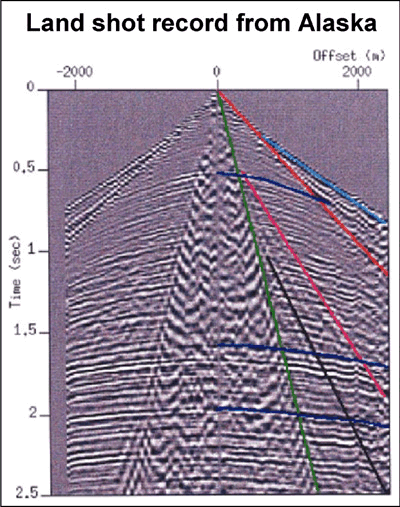
 Figure
2 – A land shot record from Alaska (courtesy of SEG). Several kinds of events,
in addition to reflections, are marked on the right side of the record,
indicating the path and wave type from source to receiver.
Figure
2 – A land shot record from Alaska (courtesy of SEG). Several kinds of events,
in addition to reflections, are marked on the right side of the record,
indicating the path and wave type from source to receiver.
Click
here for sequence of Figures 2, 5, 6.
 Figure
3 – A seismic line is acquired by rolling the shot and receivers a certain
distance forward. This gives more than one trace with the same midpoint.
Figure
3 – A seismic line is acquired by rolling the shot and receivers a certain
distance forward. This gives more than one trace with the same midpoint.
 Figure
4 – All the traces that live at the same CMP location will be processed
together as a family. Ultimately, they will be added (stacked) to make one stack
trace that lives at this location. The process of Normal MoveOut (
Figure
4 – All the traces that live at the same CMP location will be processed
together as a family. Ultimately, they will be added (stacked) to make one stack
trace that lives at this location. The process of Normal MoveOut ( NMO NMO ) helps
prepare the traces before they are added together. ) helps
prepare the traces before they are added together.
 Figure
5 – Data from Figure 2 after Normal
MoveOut processing (and air wave removal).
The blue box highlights static problems; the red box shows stretched direct
arrivals and head waves. Reflection events are flat (more or less).
Figure
5 – Data from Figure 2 after Normal
MoveOut processing (and air wave removal).
The blue box highlights static problems; the red box shows stretched direct
arrivals and head waves. Reflection events are flat (more or less).
Click
here for sequence of Figures 2, 5, 6.
 Figure
6 – Data after NMO with a 25 percent stretch mute. Note that the nasty events
in the red box of Figure 5 have been removed.
Figure
6 – Data after NMO with a 25 percent stretch mute. Note that the nasty events
in the red box of Figure 5 have been removed.
Click
here for sequence of Figures 2, 5, 6.
 Figure
7 – When the reflector is dipping, midpoints are not vertically above
reflection points. Compare Figure 4. NMO can handle this case, but breaks down
when multiple dips are present in the subsurface.
Figure
7 – When the reflector is dipping, midpoints are not vertically above
reflection points. Compare Figure 4. NMO can handle this case, but breaks down
when multiple dips are present in the subsurface.
 Figure
8. Normal MoveOut (NMO) is a process applied to pre-stack data. Here the effect
is shown on a single trace with one reflection event (left). NMO assumes the
reflection comes from a horizontal interface in the earth (center). Using a
velocity function supplied by the processor, NMO adjusts the original time (red)
to that which would have been observed at the midpoint, marked S/R. The blue
path is two-way time down and back, which must be less than the red path time.
So NMO’s job is to move the reflection event up the trace (right). Note NMO
operates on one trace at a time, which makes it inexpensive.
Figure
8. Normal MoveOut (NMO) is a process applied to pre-stack data. Here the effect
is shown on a single trace with one reflection event (left). NMO assumes the
reflection comes from a horizontal interface in the earth (center). Using a
velocity function supplied by the processor, NMO adjusts the original time (red)
to that which would have been observed at the midpoint, marked S/R. The blue
path is two-way time down and back, which must be less than the red path time.
So NMO’s job is to move the reflection event up the trace (right). Note NMO
operates on one trace at a time, which makes it inexpensive.
 Figure
9. Dip MoveOut (DMO) is a process that is applied after NMO. Since NMO assumes
the reflection comes from a horizontal bed, it is picking up only one of many
possibilities. For one trace with one reflection event, all possible travel
paths have the same length – that is, the distance from source to reflection
point to receiver is a constant. The geometrical shape with this property is an
ellipse (upper). Some of the original path possibilities are shown in red. NMO
reduces travel time based on a horizontal reflector (blue path), while DMO does
all the other cases (green). So the action of DMO (lower) is to take the NMO’d
event (blue) and broadcast it across several nearby traces (green). Since DMO
operates on several traces, it is expensive.
Figure
9. Dip MoveOut (DMO) is a process that is applied after NMO. Since NMO assumes
the reflection comes from a horizontal bed, it is picking up only one of many
possibilities. For one trace with one reflection event, all possible travel
paths have the same length – that is, the distance from source to reflection
point to receiver is a constant. The geometrical shape with this property is an
ellipse (upper). Some of the original path possibilities are shown in red. NMO
reduces travel time based on a horizontal reflector (blue path), while DMO does
all the other cases (green). So the action of DMO (lower) is to take the NMO’d
event (blue) and broadcast it across several nearby traces (green). Since DMO
operates on several traces, it is expensive.
 Figure
10. This numerical example illustrates the effect of NMO and DMO on a trace with
two spikes, or reflection events. The spikes are shown on the left surrounded by
a bunch of zero traces. The source and receiver locations are denoted by S and
R, respectively. NMO shifts the spikes up in time, but only on the same trace
(middle). DMO throws the NMO’d spike amplitude out along a curve to handle all
possible dips. This curve is called the DMO smile, or DMO ellipse, or DMO
impulse response. Notice the DMO smile only lives between the original source
and receiver positions.
Figure
10. This numerical example illustrates the effect of NMO and DMO on a trace with
two spikes, or reflection events. The spikes are shown on the left surrounded by
a bunch of zero traces. The source and receiver locations are denoted by S and
R, respectively. NMO shifts the spikes up in time, but only on the same trace
(middle). DMO throws the NMO’d spike amplitude out along a curve to handle all
possible dips. This curve is called the DMO smile, or DMO ellipse, or DMO
impulse response. Notice the DMO smile only lives between the original source
and receiver positions.
 Figure
11. This chart illustrates processing time in seconds for a small sample data
set. The relative times are important, not the size of the data set or kind of
machine used. Starting from the bottom, the processes represent (in order) a
more-or-less standard processing flow. By far the most expensive item here is
DMO. However, if we run pre-stack migration instead, it is even more expensive.
Basically, the pre-stack migration replaces NMO, DMO, stack and post-stack
migration. Due to the cost, pre-stack migration is a method to be used only when
required by strong lateral velocity variations and/or extreme structure.
Figure
11. This chart illustrates processing time in seconds for a small sample data
set. The relative times are important, not the size of the data set or kind of
machine used. Starting from the bottom, the processes represent (in order) a
more-or-less standard processing flow. By far the most expensive item here is
DMO. However, if we run pre-stack migration instead, it is even more expensive.
Basically, the pre-stack migration replaces NMO, DMO, stack and post-stack
migration. Due to the cost, pre-stack migration is a method to be used only when
required by strong lateral velocity variations and/or extreme structure.
Return
to top.
Background
Petroleum
seismology is, and always has been, changing very quickly. You might have heard
whispers about exotic topics like crosswell tomography, wavelet transforms,
cluster analysis, texture segmentation impedance inversion, geostatistical
estimation, etc. So why in this high-tech age is someone writing about something
as ancient as normal moveout? The answer involves the importance of
understanding fundamental concepts, the natural lead-in that normal moveout
provides to the juicier topic of dip moveout, and a chance to do it without any
equations.
Normal
moveout has two meanings – it is both:
By
itself, the term “moveout” goes back to the earliest days of reflection
seismology in the 1910s. In those days a seismic shot consisted of a source
(dynamite) sending waves into the earth to bounce around and return to a few
geophones. The data were preserved as wiggly lines (traces) on a rotating drum
of paper, or as dark lines on a photographic record.
The
human eye is wonderfully adept at seeing patterns and relationships in very
confusing data, e.g. recognizing a face across a crowded room full of strangers.
Early seismic records were like that – lots of noise, not much signal. But the
signals were there, and skilled interpreters could recognize them. Some of these
signal events came in straight lines across the traces; others formed curves.
But whatever the shape, each kind of signal showed a delay from trace to trace
as we move away from the source – and thus was known as moveout.
You
can talk about Normal MoveOut (NMO) all day long without mentioning migration,
but Dip MoveOut (DMO) is another matter. In fact, DMO started out with the
cumbersome-but-descriptive name “pre-stack partial migration.” That was in
1979, but at least two years earlier there was a DMO processing product on the
market. It was named DEVILISH, an acronym for “dipping event velocity
inequality licked.” You think I am making this up, but it’s true. Before
moving on, I should say something about name-dropping. Unlike NMO, the
development of DMO is very recent. The people involved are still alive and
kicking. We owe a debt of gratitude for their hard work and ingenuity, but if I
mention one name I will have to mention them all. So we shall deal here with the
concepts and not the names. We shall attempt to understand what DMO is and does,
not create a historical who’s who.
A Normal Example
A
shot record is the collection of seismic traces generated when one source shoots
into many receivers, as shown in Figure 1. In this example, the upper black line
is the acquisition surface and the lower one is the reflector. Dots below the
reflector show subsurface reflection points. Halfway between the source and a
receiver is a point on the ground called the midpoint. These are shown as black
dots above the acquisition surface Where there is no dip, the midpoint is
directly above the reflection point. As the offset (source to receiver distance)
increases, so does the travel time from source to receiver. This characteristic
delay of reflection times with increasing offset is called normal moveout.
In
Figure 2 (page 26), reflections can be seen in real data along with other kinds
of events. There are receivers on both sides of the shot in this case. The right
side has been marked-up to identify different kinds of events – direct
arrivals (p-wave, s-wave, air wave, surface wave), head waves and (a few)
reflections. The left side is uninterpreted. The reflection events have a
hyperbolic shape characteristic of normal moveout.
Return
to top.
Making the Earth Flat
So
now we know something about normal moveout, the effect. What about normal
moveout, the process? For this we will use the acronym NMO (Normal MoveOut)
since for most people this term implies the process, not the effect.
What
is NMO? The short answer is:
A
seismic processing step whereby reflection events are flattened in a common
midpoint gather in preparation for stacking. (If this makes sense then you can
move along to the second part of this article. Otherwise, read on.)
A
seismic line is generated by “rolling” the shot and receivers forward a
certain distance and firing again. As shown in Figure
3, this generates a second
shot record which partially overlaps the first. Note that six of the seven
reflection points from the blue shot were also reflection points for the red
shot. This occurs by design and is called Common MidPoint (CMP) shooting.
As
the shots roll along, there will be many source-receiver pairs with the same CMP
location, and the CMP fold is the total number of traces that live at any given
CMP (Figure 4). CMP fold can vary from as few as
six (low-fold land 3-D) up to several hundred (2-D marine). The reason for
gathering multifold data is that we get redundant information about the
reflection point down in the earth, and this redundancy can be used to reduce
noise and create a more reliable image. Our goal is to eventually process all
these traces as a family and add them together (CMP stack) to make one trace
that lives at this CMP location.
NMO
is aimed at removing the hyperbolic curvature in reflection events. Basically,
it is removing the effect of offset. If this is done properly, then the
reflection should come in at the same time for all offsets (since we have
removed any travel time delay due to offset). In short, reflection events should
be flat after NMO.
Figure
5 shows the data after NMO processing (and air wave removal). In this case, we
see the events are pretty well flattened by NMO, but there are a couple of
interesting areas. The blue box shows some disturbing behavior along a flattened
reflection. This has nothing at all to do with NMO, but is related to lateral
changes in the near surface layers (termed a static problem).
The
red box shows what NMO does to the direct arrivals. Since these were linear and
not hyperbolic, NMO has not flattened them. Also, note how fat (not flat) these
events look after NMO. This is because NMO actually operates by stretching the
trace – and the shallower something is, the more it stretches.
Since
our goal is to eventually flatten all these traces and add them together to make
one trace, keeping this kind of stuff would wipe out shallow reflections. It
needs to go. We get rid of these events by muting – which is nothing more than
replacing the offending data with zeros. We could do this by hand, but a seismic
line may contain many thousands of CMP gathers.
It
turns out we can let NMO itself do the muting for us. The idea is to keep track
of how much stretch NMO is doing to the trace. The stretch changes down the
trace – biggest at the top, smallest at the bottom. So the idea of an NMO
stretch mute is to set a limit on how much stretch we are going to allow. If the
stretch gets bigger than our limit, then the data values are replaced by zeros
in that part of the trace. Figure 6 shows the result of allowing a 25 percent
stretch in the NMO process.
What About Dips?
At
this point more than one astute reader is saying, “Yeah, yeah, you academic
types are all alike – ignoring the real world. What about dipping beds?”
Figure 7 gives a hint of things to come. The basic problem is that when the bed
dips, midpoints are not vertically above reflection points. Furthermore, the
reflection points become unevenly spaced along the reflector.
The
fact is that NMO has a constant dip assumption built in. If every bed were
dipping at the same angle, say 23 degrees, it turns out we could do NMO just
fine. The real problem comes where there are many dips in the subsurface. In
this case, NMO acts like a dip filter – preferentially passing some dip the
processor chooses while suppressing others. This was particularly notorious in
places like the Gulf of Mexico, where gently dipping beds often meet steep salt
domes. You could do NMO in such a way as to get a good image of one or the
other, but not both. This was the situation up until about 1981 or 1982. Then
something new came on the scene. It was called – you guessed it – dip
moveout.
Return
to top.
Dip MoveOut
In
the field, a source and receiver are located, say, 3,000 meters apart (the
offset) and a trace is recorded. This is pre-stack data. From the notes above,
we know that NMO lives to remove offset from pre-stack data. In the computer, we
adjust this trace to simulate one that would have been recorded with no effect
at a point half-way between the source and receiver (the midpoint). This new
trace is a zero-offset trace, and adding (stacking) all such traces that live at
this midpoint yields a stack trace. All the stack traces plotted side-by-side
form the stack section, which is raw material for post-stack migration
processing.
Figure
8 illustrates the NMO idea. On the left is a field trace with some arbitrary
offset and one reflection event. NMO assumes the reflection comes from a
horizontal interface is shown in the middle (inset) figure. This is an important
and restrictive assumption. The NMO correction adjusts observed travel time (red
path) to midpoint zero-offset travel time (blue path). So after NMO, the event
is moved up in time. Technically, we are changing time coordinate from raw time,
t, to NMO time, tn.
But
what if the interface is not horizontal? It is tempting to think that the
reflector could be anywhere and still be consistent with the observed travel
time. But this is not the case. Assume that the original travel time is 1.0
second, and we know the velocity is 3,000 m/s. The total distance traveled has
got to be 3,000 meters. So all valid reflector positions have one thing in
common: The total distance from source to reflection point to receiver is
constant, namely 3,000 meters. Thinking back to Geometry 101, this is just the
definition of an ellipse with the source and receiver at each focus.
Figure 9
shows such an ellipse. Remember the goal is to remove offset and thus create a
zero-offset section. NMO gives one of many possibilities; DMO gives all the
rest. In Figure 9, some of the possible original travel paths are shown (red),
along with the single travel path after NMO (blue) and the many travel paths
after DMO (green).
From
Figure 8, we saw that NMO is a process that takes one trace in and gives one
trace out. DMO is different. One trace into DMO generates many traces out –
all of which live between the original source and receiver locations. This is
illustrated in Figure 9 (lower) and Figure
10.
In
Figure
10, we have a panel of data containing only two spikes of amplitude on
one trace (left panel). The other traces are there, but empty. NMO moves the
spike up on the same trace (middle panel). DMO then throws the spike out along a
curve, which lives between the source and receiver (right panel). This is
sometimes called the DMO smile. Since it comes from a spike or impulse on the
input data, it is also called the DMO impulse response.
Now
here is some magic. By creating the DMO smile, all possible dips are handled
simultaneously. We do not need to know what the dip is in the earth – by
processing all traces with DMO, the actual reflections will emerge because they
are tangent, at some point, to DMO smiles. Also, DMO does not depend on the
velocity, so long as the velocity is constant. While not strictly true, this is
one of the things that got everyone initially excited about DMO. And its weak
dependence on velocity is one reason it is still so widely used. Anyway, it is
unlike NMO and migration, which always need velocity information, and are quite
sensitive to it. Another big selling point is that NMO+DMO, rather than NMO
alone, passes all dips into the stack section. This gives more raw material for
migration to work with in creating a final migrated image.
Since
DMO spreads things out across traces, it is much more expensive than NMO, which
only shifts things up on one trace. Even so, NMO+DMO is still cheaper than
pre-stack migration. Figure 11 gives some representative run times for these,
and other, processes.
Conclusion
Here
is the bottom line: If structure and velocity variation are not too nasty in an
area, we can get away with a traditional processing sequence:
NMO + DMO +
Stack + PostStackMigration.
In this equation,
“+” means “followed by.” However, if things get really tough down there
(e.g., subsalt), this sequence breaks down and fails to give a good image. In
this case we are compelled to do one grand process called pre-stack migration.
In
fact, DMO was originally invented to complete the following equality under mild
subsurface conditions:
PreStackMigration =
NMO + ? +Stack + PostStackMigration. + ? +Stack + PostStackMigration.
The
“?” turned out to be DMO – and is used world-wide every day.
Return
to top.
|