GCPolygonal Fault Expression in 3-D Seismic Data*
Esther Ali¹, Emma Gibbons¹, Juan Martinez-Munoz¹, Karl Schleicher², Dennis Cooke³, and Kurt J. Marfurt¹
Search and Discovery Article #41589 (2015)
Posted March 20, 2015
*Adapted from the Geophysical Corner column, prepared by the authors, in AAPG Explorer, February, 2015, and entitled "Fault Finding? Access to 3-D Data Always Helps". Editor of Geophysical Corner is Satinder Chopra ([email protected]). Managing Editor of AAPG Explorer is Vern Stefanic. AAPG © 2015
¹University of Oklahoma, Norman, Oklahoma, USA ([email protected])
²University of Texas at Austin, Bureau of Economic Geology, Austin, Texas, USA
³University of Adelaide and ZDAC Geophysical Technologies, Glen Osmond, Australia
Access to modern 3-D seismic data is critical to educating the next generation of sedimentologists, stratigraphers, structural geologists and geophysicists who envision a career in the petroleum industry. While suffering from limits to vertical and lateral resolution, 3-D seismic volumes generate a more complete image of the subsurface than 2-D outcrops of limited vertical and lateral extent.
At the graduate level, geoscience students are calibrating seismic data with outcrop analogues, putting them within a depositional, diagenetic or tectonic framework and developing new workflows based on new seismic attributes, clustering and 3-D visualization. Until recently, there have been very few seismic data volumes available for student education and research. There are several small data volumes acquired with U.S. government funding (Stratton Field, Teapot Dome, Waha) and few larger data volumes that have been released from the Netherlands (F3) and Norway (Gulfaks).
Working with individual operators and service companies, students at the University of Oklahoma have had access to a fairly rich assortment of proprietary 3-D land seismic surveys licensed for a specific project. Other universities without such relationships face a greater challenge. For all of us, data licenses to deepwater surveys are even more problematic, with the data being owned either by multiple partners or acquired as a spec survey where the goal is to sell the data as often as possible.
Access to petroleum exploration data, however, is more open in Australia and New Zealand, where seismic and well data are released to the public after a few years. New Zealand Petroleum and Minerals (NZPM) is the governmental agency in New Zealand responsible for data compilation and release. Karl Schleicher and AAPG member Dennis Cooke have worked with NZPM and the SEG to place some 3-D seismic volumes from the Taranaki, Great South and Canterbury basins in an SEG-sponsored public repository for use by universities and the research community at large. These volumes contain spectacular images of turbidites, mass transport complexes, syneresis and volcanic intrusives.
In this article we focus on the seismic expression of polygonal faulting seen in NZPM's Waka 3-D Great South Basin survey, used by the first three authors as a final project in a 3-D seismic interpretation class.
|
♦General statement ♦Figures ♦Examples ♦Conclusion ♦Acknowledgment ♦Reference
♦General statement ♦Figures ♦Examples ♦Conclusion ♦Acknowledgment ♦Reference
♦General statement ♦Figures ♦Examples ♦Conclusion ♦Acknowledgment ♦Reference
♦General statement ♦Figures ♦Examples ♦Conclusion ♦Acknowledgment ♦Reference |
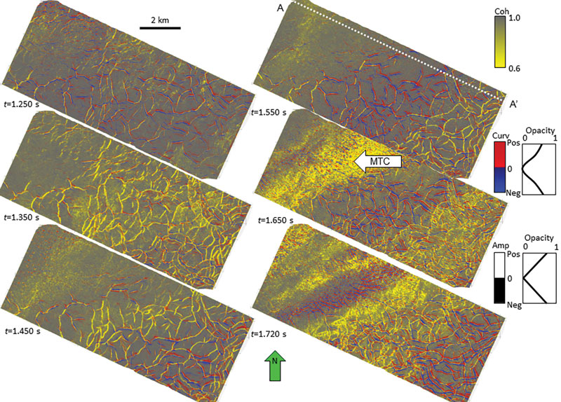
Polygonal faulting is common in many surveys and has been well documented in a recent AAPG Bulletin article by Jackson et al. (2014) on a deepwater North Sea survey. In general, tectonically generated polygonal faulting will be through-going, while syneresis (less accurately called "shale dewatering") shows similar patterns that are constrained to fall within discrete shale formations. Interpreters routinely use coherence to map faults on time slices and seismic amplitude on vertical slices. Here, we show the value of using multi-attribute display to better quantify the seismic expression of such faults. Edges are best seen using a monochromatic color bar, with a simple gray scale being the most popular means to display coherence. While a gray scale works well when displayed on top of seismic amplitude using a red-white-blue color bar, it works poorly when displayed on top of seismic amplitude using black-gray-white color bar. For this reason, we've chosen the monochrome yellow-to-gray color bar shown in Figure 1 to display coherence as the "background" attribute. Next we co-render most-positive and most-negative curvature using the binary red and blue color bar, and show the amplitude of the anomaly through the use of opacity, with a curvature value of zero (planar features) being rendered as transparent. Finally, on the vertical slice we display seismic amplitude using a binary black and white color bar. Again, using opacity, we set zero values of amplitude to be transparent, and high positive (white) and high negative (black) values of amplitude to be more opaque. In general, synclinal features in Figure 1 appear as blue and anticlinal features as red, though we need to remember that curvature is a 3-D measure, and a synclinal expression in this vertical slice may be anticlinal in the perpendicular direction. For this reason, on the footwall side of many of the faults we observe a red positive curvature anomaly, while on the hanging wall side we observe a blue negative curvature anomaly. The faults in this vertical slice have a distinct offset, giving rise to a yellow coherence anomaly – suggesting the rock is relatively brittle. A very common pattern then is red-yellow-blue, with the curvature anomalies bracketing the coherence anomaly. Qualitatively, curvature provides a measure of the width of the damage zone. The broad yellow low coherence anomaly seen on the time slice corresponds to a mass transport complex (MTC), which are quite common in the NZPM surveys. Given this mental calibration, we turn to Figure 2, which shows a suite of time slices, beginning relatively shallow at t=1.250 s and increasing at 0.5 s intervals, with the exception of the last image at t=1.720 s. The time slice of Figure 1 at t=1.650 with the MTC is repeated in these images, but now oriented from south to north. The water bottom is at about t=0.800 s. Note the change is fault expression at the different time slices. At t=1.250 s, we note the red-yellow-blue pattern seen on the previous vertical slices. However, at t=1.350 s, most of the faults give rise to a strong coherence anomaly, with little curvature expression. We suspect the lithology at this level is more brittle. In contrast, near the center of the slice at t=1.550 s, we see primarily curvature anomalies in red and blue, with fewer coherence anomalies, suggesting the lithology may be more ductile. As we progress further down section to t=1.720 s, we see a change in the size of the polygonal faulting, with smaller polygons seen in the west-central part of the survey and larger polygons in the southeast part of the survey. At present, we do not know why this change occurs. As in most surveys, we lose spectral resolution as we go deeper. In Figure 3, we show a time slice at t=1.970 s. The somewhat "wormy" pattern seen on the time slice indicated by the white block arrow of red-yellow-blue-yellow-red appears "artificial." However, closer inspection of the vertical slice cutting it (left image in Figure 3) shows that it is a small graben, separated by adjacent horst blocks by (yellow) faults. The worminess of the fault pattern may be real; however, one must also consider the cumulative effects of fault-shadow velocity pull up and push down in the overburden. This work is highly preliminary, with the exercises done as a class project by first-time seismic interpreters. Our interpretation may be full of faults – however, we think the reader will agree that we have no fault with NZMP for providing us at OU and other universities around the world, access to their data. We thank the New Zealand Petroleum and Minerals (NZPM) for providing data. Jackson, Christopher A.-L., Daniel T. Carruthers, Seshane N. Mahlo, and Omieari Briggs, 2014, Can polygonal faults help locate deep-water reservoirs?: AAPG Bltn, v. 98, p. 1717-1738. |