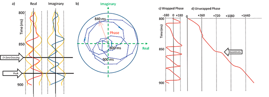
Figure 1. (a) The “complex” trace composed of the original measured trace, d(t), (the real part, in red) and its Hilbert transform, dH(t), (the imaginary part, in blue) extracted from the survey shown in Figure 2 and Figure 3. The envelope and its reverse are plotted in orange. Note how it “envelopes” the real and the imaginary trace (and indeed any phase-rotated version of the trace). (b) The complex trace plotted parametrically against time on a complex plot. Each time sample can also be represented in polar coordinates as a magnitude and phase, with phase being measured counterclockwise from the real axis. (c) The wrapped phase computed as φ=ATAN2[dH(t),d(t)]. The definition of the arctangent gives rise to discontinuities at ±1800. (d) The unwrapped phase, retaining only discontinuities associated with waveform interference (geology and crossing noise).