|
Statement
of Problem
A
problem that has always plagued geologists and interpreting geophysicists
is the fact that seismic data resemble a cross-section of the earth, but
are displayed in  time time rather than depth. To tie well control to seismic,
well logs must be scaled to time, using check shot surveys or velocity
functions derived from other means. The vertical exaggeration changes with
depth (because velocity usually increases with depth), thus distorting the
perspective and changing the apparent dip of fault planes, etc. rather than depth. To tie well control to seismic,
well logs must be scaled to time, using check shot surveys or velocity
functions derived from other means. The vertical exaggeration changes with
depth (because velocity usually increases with depth), thus distorting the
perspective and changing the apparent dip of fault planes, etc.
These
problems, however, are minor compared with the structural distortions that
occur when velocity varies laterally as well as with depth. A solution to
these problems exists in the development of pre-stack depth
migration.
Figure
Captions
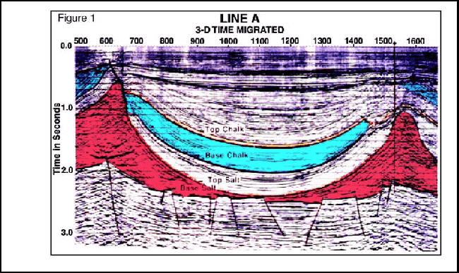
 Figure
1. A 3-D time-migrated line across two salt domes. Note severe distortion
of base salt between S.P. 500 and 700. A well was drilled near S.P. 1520. Figure
1. A 3-D time-migrated line across two salt domes. Note severe distortion
of base salt between S.P. 500 and 700. A well was drilled near S.P. 1520.
Click
here for sequence of Figures 1 and 2.

Figure
2. A 2-D prestack migrated line of the same area as in Figure 1,
providing
improved imaging beneath the left salt dome, movement of fault image near
the well, beneath the right salt dome. The well is now down thrown to the
fault.
Click
here for sequence of Figures 1 and 2.
Figure
3. Faulting that displaces beds with anomalous velocity. Figure 3a shows a
fault shadow model; Figure 3b is an example of poststack migration of
synthetic data.
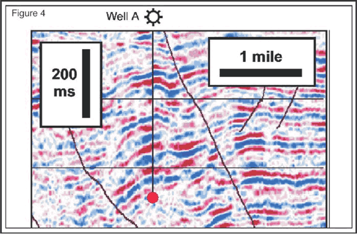
 Figure
4. Seismic line in South Texas, with poststack time migration, for
comparison with same line with prestack depth migration (Figure
5). Figure
4. Seismic line in South Texas, with poststack time migration, for
comparison with same line with prestack depth migration (Figure
5).
Click
here for sequence of Figures 4 and 5.

Figure
5. Seismic line in South Texas, with prestack depth migration, for
comparison with same line with poststack time migration (Figure.
4).
Click
here for sequence of Figures 4 and 5.
Applications
One
of the principal motivators behind development of pre-stack depth
migration was the desire to image seismic reflectors beneath salt
structures. The abrupt velocity contrasts between the salt and adjacent
sediment – coupled with the sometimes radical structural features
associated with salt tectonics – produced severe distortions in the
seismic travel times. The result is frequently a very poor stack and time
pull-ups in the events that do stack.
Time
migration incorrectly migrates the distorted events because of the rapidly
varying lateral velocities. An example of this from the Southern North Sea
gas basin is shown in figures 1 and 2.
Figure 1 is the 3-D time migrated
line from a survey across two salt structures. The objective is the
Rotliegendes sand beneath the Zechstein salt. The greatest velocity
contrast is actually between the Cretaceous Chalk that has been forced
upward by the salt movement, and the overlying Tertiary clastics. It is
this Tertiary-Cretaceous boundary and the structure on it that produce the
greatest distortion. Severe distortions can be seen in the Base Salt/Top
Rotliegendes reflector beneath each of the structures. The event actually
criss-crosses in a reverse “bow-tie” beneath the structure on the
left. An apparent fault is seen beneath the structure on the right.
Prestack
depth migration, shown in Figure 2, reveals a very different picture. The
“bow-tie” under the left structure has been unraveled, revealing a
much clearer image that has moved somewhat. Note that the well that was
drilled with the intention of reaching the upthrown side of the fault (Figure
1), in fact, entered the downthrown side, as seen in the depth
image (Figure 2), and reached the base of salt at exactly the depth
indicated in the depth section (about 300 meters low to prognosis, as
interpreted from the time section).
Another
more subtle example of the value of prestack depth migration is the
“fault shadow” problem. Figure 3 illustrates, with model data, what
can happen if faulting displaces beds with anomalous velocity, thus
causing abrupt lateral changes. The raypaths of various offsets passing
through the faulted zone are disrupted such that:
·
They stack poorly.
·
The stacked traces have severe
time distortion.
Such
distortion can easily be interpreted as structure and/or secondary
faulting. Figures 4 and 5 show a comparison of a seismic line in South
Texas, with time migration and prestack depth migration. The effect is
most clearly seen in the two circled areas, where the time section
indicates folded beds that are much more planar in the depth section.
False structures could very easily be interpreted on the time data.
Other
problem areas where depth migration can help include overthrust faults,
channel fills, reefs, and karsted or eroded carbonate in the section above
the zone of interest. In short, any time the objective lies beneath strata
that have been disrupted by faulting, diapirism, etc. or show significant
structural dip or where there are significant lateral variations in the
overburden velocity, depth migration can be useful.
Summary
There
are two reasons for performing depth migration prestack, rather than after
stack:
·
The velocity model can be derived
directly from the data, usually with more accuracy than from stacking
velocity or extrapolated well control.
·
The stack itself is disrupted and
degraded beneath velocity anomalies. Prestack depth migration, with a
correct model, can improve the stacked image.
Deriving and refining the velocity model is an
iterative process, requiring numerous preliminary migrations and analysis
cycles. Because of this, depth migration is expensive compared to other
data processing procedures. However, it is cheap compared to the cost of
drilling dry holes (see Figures 1 and 2)! is expensive compared to other
data processing procedures. However, it is cheap compared to the cost of
drilling dry holes (see Figures 1 and 2)!
Return
to top.
|