![]() Click to view article in PDF format.
Click to view article in PDF format.
A Practical Approach to Seismic Imaging of Complex Geology*
By
Matthew Brzostowski1 and Todd Jones2
Search and Discovery Article #40057 (2002)
*Adapted for online presentation from the article by the authors in AAPG Explorer (April, 2000), entitled “Complexities Can Be Mind-Bending.” Appreciation is expressed to the authors and to M. Ray Thomasson, former Chairman of the AAPG Geophysical Integration Committee, and Larry Nation, AAPG Communications Director, for their support of this online version.
1Houston, Texas (713-469-1311)
2Houston, Texas
|
|
General StatementThe biggest distinction between geology and geophysics can probably be broken down into the different domains from which they both start their work. The geologist works in terms of spatial coordinates and depth, with perhaps the roadcut epitomizing the best example of his world view. Depth is also how he makes use of his interpretation results, i.e. a well is drilled to a certain depth. The geophysicist, however, deals with information recorded in time. His job in seismic processing is to transform this information in time into depth for the geologist to make his maps and calculate where to drill. The geophysicist works in time because of the nature of seismic exploration. A source is initiated at some location and sensors record the subsequent reflections as a function of time.
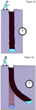
Figure 1b. Complications of translating time into distance where the well is not vertical.
Analogies and ExamplesThe problem is not unlike the scenario depicted in Figure 1a: Here we have a person determining the depth of his water well by dropping a rock into it and recording the time for the splashing sound to come back. After some mathematical manipulation - and knowing the speed of sound in air - the person can translate time into depth. This sounds simple enough, but we made assumptions about the rock traveling straight down and the sound traveling straight back up to our ears. If the well is not vertically straight but deviated (Figure 1b), then we have a more complicated problem to solve. This is the nature of seismic exploration: We record the strength of seismic reflections, and we can assume they all come from directly below the surface, but more likely the reflections come from anywhere in some three dimensional subsurface location around our surface position. Figure 2a shows more clearly the issue. Reflected energy from a subsurface point will travel to our surface receivers in a straight line if the velocity field is constant. It would be a simple and straightforward process to compute the location of the subsurface point if we knew this velocity field. However, the issue becomes more complicated when we acknowledge that seismic energy bends according to Snell’s law when the velocity changes in the subsurface as shown in Figure 2b. Obviously, there is a lot of velocity contrast in complex geologic regimes. This ray bending is not unlike light bending as it travels through water and air as depicted in Figure 3. The resultant bent rays can lead to a gross misinterpretation of what is in the glass if we do not account for it. That is the goal of seismic imaging; accounting for the complicated velocities in the subsurface that will distort our interpretation, especially in terms of where features are actually located. Figure 4 shows this distortion due to velocity contrasts quite clearly. In both cases we are looking for the oil trap depicted by the black shape. In one case, on the left in Figure 4, we need only deal with the relatively minor velocity contrast between the water column and the subsurface when imaging the seismic reflections. In the second case, in Figure 4 (right), the oil trap is located below salt, so the seismic reflections will be bent sharply as they travel through the salt body. Snell’s law tells us we will have more ray bending with more velocity contrast. Salt normally has a 2:1 velocity contrast with surrounding sediments, which amounts to a great deal of ray bending. If we do not honor this ray bending, we could spatially mislocate the oil trap as depicted by the gray shape to the left of the actual location of the oil trap in Figure 4 (right). Specification of Velocity field One of the means we have for controlling the processing of seismic data and the eventual placement of events comes from the specification of a velocity field. We normally use the timing of seismic reflections as a function of spatial position and offset to determine this velocity field. However, we can make approximations to the velocity field when it comes to imaging the seismic data. There are two broad classes of imaging algorithms available to the geophysicist. One class has historically been referred to as time migration, while the other class has been referred to as depth migration. The names are confusing because of the implication as to the domain the final images are in. However, it is possible to convert seismic data from time to depth with simple vertical shifts of the data. The main difference in the algorithms comes about in how they approximate the velocity field. Time migration velocity fields will not honor lateral velocity changes, although they can pick up vertical changes, as depicted in Figure 5 (right). Time migration algorithms do this for the sake of faster computation speed and less image sensitivity to the velocity model. Depth migration velocity fields look more like the geology you are trying to image, as depicted in Figure 5 (left). Notice how the velocity wedge is accurately portrayed, while the time migration velocity field, Figure 5 (right), is a laterally averaged representation. The price for the accuracy, however, is more expense - and there is a greater need to determine the velocity field accurately. Imaging algorithms are available, as are mechanisms to build the velocity model |
 Figure
1a. Determination of the depth of a water well by translating time into
distance.
Figure
1a. Determination of the depth of a water well by translating time into
distance.
 Figure
3: A simple example of light rays bending across the air-water surface.
Figure
3: A simple example of light rays bending across the air-water surface.