GCSpectral Balancing Can Enhance Vertical Resolution*
Kurt J. Marfurt¹ and Marcilio C. de Matos²
Search and Discovery Article #41357 (2014).
Posted May 31, 2014
*Adapted from the Geophysical Corner column, prepared by the author, in AAPG Explorer, May, 2014 and entitled "Am I Blue? Finding the Right (Spectral) Balance".
Editor of Geophysical Corner is Satinder Chopra ([email protected]). Managing Editor of AAPG Explorer is Vern Stefanic.
¹University of Oklahoma, Norman, Oklahoma ([email protected])
²Sismo Research, Rio de Janeiro, Brazil
Seismic interpreters have always desired to extract as much vertical resolution from their data as possible – and that desire has only increased with the need to accurately land horizontal wells within target lithologies that fall at or below the limits of seismic resolution. Although we often think of increasing the higher frequencies, resolution should be measured in the number of octaves, whereby halving the lowest frequency measured doubles the resolution.
There are several reasons why seismic data are band-limited. First, if a vibrator sweep ranges between 8 and 120 Hz, the only "signal" outside of this range is in difficult to process (and usually undesirable) harmonics. Dynamite and airgun sources may have higher frequencies, but conversion of elastic to heat energy (intrinsic attenuation), scattering from rugose surfaces and thin bed reverberations (geometric attenuation) attenuate the higher frequency signal to a level where they fall below the noise threshold. Geophone and source arrays attenuate short wavelength events where individual array elements experience different statics.
Processing also attenuates frequencies. Processors often need to filter out the lowest frequencies to attenuate ground roll and ocean swell noise. Small errors in statics and velocities result in misaligned traces that when stacked preserve the lower frequencies but attenuate the higher frequencies.
Currently there are two approaches to spectral enhancement. More modern innovations that have been given names such as "bandwidth extension," "spectral broadening" and "spectral enhancement," are based on a model similar to deconvolution, which assumes the Earth is composed of discrete, piecewise constant impedance layers. Such a "sparse spike" assumption allows one to replace a wavelet with a spike, which is then replaced with a broader band wavelet that often exceeds the bandwidth of the seismic source.
Model-based processing is common to reflection seismology and often provides excellent results – however, the legitimacy of the model needs to be validated, such as tying the broader band product to a well not used in the processing workflow. We have found bandwidth extension algorithms to work well in lithified Paleozoic shale resource plays and carbonate reservoirs. In contrast, bandwidth extension can work poorly in Tertiary Basins where the reflectivity sequence is not sparse, but rather represented by upward fining and coarsening patterns.
In this article, we review the more classical workflow of spectral balancing, constrained to fall within the source bandwidth of the data. Spectral balancing was introduced early in digital processing during the 1970s and is now relatively common in the workstation environment.
|
|
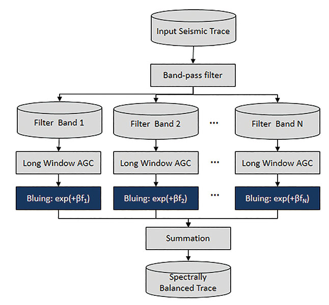
As summarized in Figure 1, the interpreter decomposes each seismic trace into a suite of 5-10 overlapping pass band filtered copies of the data. Each band-passed filtered version of the trace is then scaled such that the energy within a long (e.g. 1,000 ms) window is similar down the trace. This latter process is called automatic gain control, or AGC. Once all the components are scaled to the same target value, they are then added back together, providing a spectrally balanced output. A more recent innovation introduced about 10 years ago is to add “bluing” to the output. In this latter case, one stretches the well logs to time, generates the reflectivity sequence from the sonic and density log and then computes its spectrum. Statistically, such spectra are rarely "white," with the same values at 10 Hz and 100 Hz, but rather "blue," with larger magnitude spectral components at higher (bluer) frequencies than at lower (redder) frequencies. The objective in spectrally balancing then is to modify the seismic trace spectrum so that it approximates the well log reflectivity spectrum within the measured seismic bandwidth. Such balancing is achieved by simply multiply each band-pass filtered and AGC'd component by exp (+βf), where f is the center frequency of the filter and β is the parameter that is obtained from the well logs that varies between 0.0 and 0.5 (black boxes in Figure 1). There are several limitations to this classic workflow:
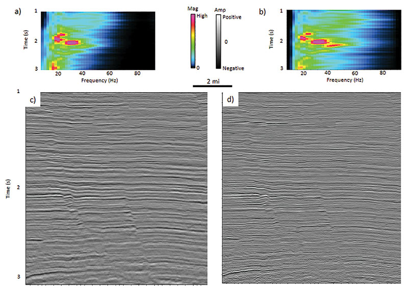
A fairly common means of estimating the spectrum of the signal is to cross-correlate adjacent traces to differentiate that part of the signal that is consistent (signal) and that part that is inconsistent (random noise). One then designs the spectral balancing parameters (AGC coefficients) on the consistent part of the data. Unfortunately, this approach is still not amplitude friendly and can remove geology if the spectra are not smooth. Figure 2 illustrates a more modern approach that can be applied to both post-stack and pre-stack migrated data volumes. First, we suppress crosscutting noise using a structure-oriented filtering algorithm, leaving mostly signal in the data. Next, the data are decomposed into time-frequency spectral components. Finally, we compute a smoothed average spectrum. If the survey has sufficient geologic variability within the smoothing window (i.e. no perfect "railroad tracks"), this spectrum will represent the time-varying source wavelet. This single average spectrum is used to design a single time-varying spectral scaling factor that is applied to each and every trace. Geologic tuning features and amplitudes are thus preserved. We apply this workflow to a legacy volume acquired in the Gulf of Mexico: Figure 3a and Figure 3b show the average spectrum before and after spectral balancing. Figure 3c and Figure 3d show a representative segment of the seismic data where we see the vertical resolution has been enhanced. |