![]() Click to view article in PDF format.
Click to view article in PDF format.
GCImpedance Inversion May Help Characterize Reservoir*
Satinder Chopra1and Ritesh Kumar Sharma1
Search and Discovery Article #41099 (2012)
Posted December 17, 2012
*Adapted from the Geophysical Corner column, prepared by the author, in AAPG Explorer, December, 2012, and entitled "A Solid Step Toward Accurate Interpretations". Editor of Geophysical Corner is Satinder Chopra ([email protected]). Managing Editor of AAPG Explorer is Vern Stefanic. AAPG©2012
1 Arcis Corp., Calgary, Canada ([email protected])
In the November 2012 Geophysical Corner we discussed the unsupervised seismic waveform classification method, which provides qualitative information on lithology in terms of facies variation in a given subsurface target zone. While this information is useful, more work needs to be done for characterizing such formations of interest in terms of porosity and fluid content. For this purpose, impedance inversion of seismic data could be used, which essentially means transforming seismic amplitudes into impedance values. Here we discuss here such impedance characterization of the formations of interest.
|
|
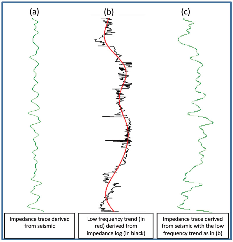
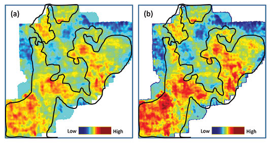
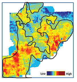
Seismic signals have a narrow frequency bandwidth, say 8-80 Hz. Frequencies below 8 or 10 Hz are lost either by bandpass filtering circuits in the recording instruments or while processing of seismic data to eliminate the low frequency noise usually present in the data. Sonic logs, on the other hand, have a very broad frequency bandwidth, extending from 0 to well over many kilohertz. While the high frequencies show the high-resolution information on the log, the low frequencies exhibit the basic velocity structure or the subsurface compaction trend. As these low frequencies are not present in the seismic data, the impedance traces derived from the seismic do not exhibit the compaction trend that the impedance logs do. When seismic data are transformed into impedance values, the low frequency trend usually is added from outside - say, from the available impedance logs. By doing so, the derived impedance values will have a range of values similar to the value range exhibited by the impedance log curves. Such a method is termed as absolute acoustic impedance inversion. In Figure 1, the addition of the low-frequency trend is demonstrated to the inverted impedance trace from seismic. Sometimes it is not possible to determine the low frequency trend accurately, which possibly could be due to the unavailability of the log data. In such cases, the derived impedance range will be devoid of the compaction trend, but would still exhibit the relative variation of the impedance values. Such a method is termed as relative acoustic impedance inversion. In the November 2012 Geophysical Corner we discussed the seismic waveform classification method for describing the facies variation of Middle Jurassic Doig sandstones in Western Canada. We pick up the same example to determine the changes of impedance in the Doig sandstones in a lateral sense, which would be reflective of the porosity changes. In Figure 2a we show a horizon slice from the relative acoustic impedance volume derived from the input data volume. Within the sand boundary (in black), there are variations in impedance. We also computed the absolute acoustic impedance on the same volume, which is shown in Figure 2b. Though the overall impedance pattern still appears more-or-less the same, there is a significant variation in the impedance (red color) within the sand boundary. The May 2008 Geophysical Corner described a thin-bed reflectivity inversion method that outputs a reflectivity series - and demonstrates that the apparent resolution of the inversion output is superior to the resolution of the input seismic data used to generate the reflectivity response. This aspect makes the method ideal for detailed delineation and characterization of thin reservoirs. We derived the reflectivity from the seismic data used for generating the impedance displays in Figure 2, and then generated relative acoustic impedance from it. The result is shown in Figure 3, where the impedance variation exhibits a pattern that is more focused than the impedance variation in Figure 2a and similar to that in Figure 2b – but superior. The main reason for this is probably the absence of the seismic wavelet in the data used to derive the relative acoustic impedance in Figure 3. Impedance inversion on highly resolved seismic data retrieved in the form of reflectivity is useful for making accurate interpretations, and so proves advantageous. We thank Arcis Seismic Solutions for permission to present this work. |
 General statement