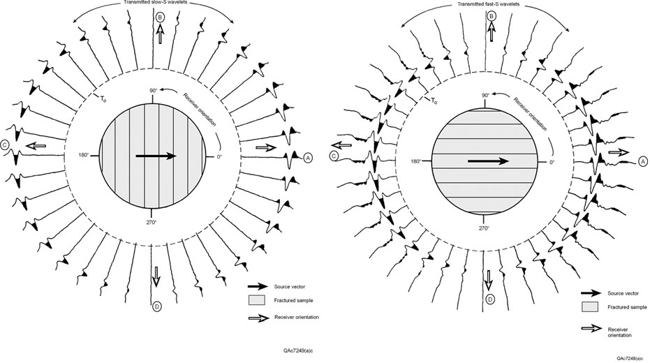
Figure 3. Data acquired using the test arrangement illustrated on Figure 2 to simulate S-wave propagation through a fractured medium. (a) The illuminating S-wave displacement vector is parallel to the test-sample fractures to simulate fast-S propagation. As the source stays fixed on one end of the sample, the receiver at the opposite end of the sample is rotated at angular increments of 10 degrees relative to the positive-polarity orientation of the source displacement vector. Every transmitted response is a fast-S wavelet. The dashed circle labeled T0 defines time zero. Arrowheads define the positive-polarity ends of the source and receiver elements. (b) The same test repeated with the illuminating S-wave displacement vector oriented perpendicular to fractures to simulate the propagation of a slow-S mode. Every transmitted response is a slow-S wavelet. Note how much longer the travel times are for wavelets polarized normal to fractures than they are for the wavelets polarized in 3a that are polarized parallel to fractures.