![]() Click to view article in PDF
format.
Click to view article in PDF
format.
GCSeismic Model for Monitoring CO2 Sequestration*
Bob Hardage1 and Diana Sava1
Search and Discovery Article #40423 (2009)
Posted May 26, 2009
*Adapted from the Geophysical Corner column, prepared by the authors, in AAPG Explorer, May, 2009, and entitled “Seismic Steps Aid Sequestration”. Editor of Geophysical Corner is Bob A. Hardage. Managing Editor of AAPG Explorer is Vern Stefanic; Larry Nation is Communications Director.
1Bureau of Economic Geology, The University of Texas at Austin (mailto:[email protected])
Sequestration of CO2 in sealed brine is an important issue in industrialized countries that are concerned about the impact of excessive atmospheric CO2 on the environment. A general consensus is that long-term seismic monitoring of injected CO2 will be essential for successful CO2 sequestration programs. In this column we consider the P-wave reflectivity associated with tracking a CO2 plume in one reservoir considered for CO2 sequestration.
|
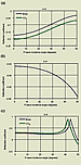
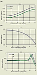
The physical properties of injected CO2 that affect seismic imaging are its density and acoustic propagation velocity at the pressure and temperature of its host medium. Because CO2 has a shear modulus of zero whether it is a gas or a liquid, shear-wave velocity in CO2 is zero. The only velocity that has to be known for seismic modeling purposes is VP, the propagation velocity of the P-wave mode in CO2. The density and P-wave velocity of CO2 over a range of pressure and temperature conditions are defined by the curves displayed in Figures 1 and 2 , respectively.
An Earth model that defines reflecting interfaces at the top and base of the sandstone reservoir and at the fluid interface between CO2 and brine internal to that reservoir is shown as Figure 3 . From available log data at this site, the Earth layers have the following petrophysical properties:
Sealing carbonaceous shale: Δtp = 65 μs/ft, ρ = 2.633 gm/cm3.
Reservoir sandstone: Δtp = 80 μs/ft, ρ = 2.357 gm/cm3, Φ = 22 percent.
Granite basement: Δtp = 55 μs/ft, ρ = 2.70 gm/cm3.
The sandstone reservoir is at a depth of 6,000 feet; it is important to define the depth of the injection interval in order to determine the temperature and hydrostatic pressure that act on the sequestered CO2. This temperature and pressure, in turn, specify the density and VP values that should be used to describe the seismic properties of the in situ CO2 (Figures 1 and 2). A factor of 0.433 psi/ft was used to convert target depth to hydrostatic pressure. In utilizing the curves in Figures 1 and 2 , the in situ temperature was assumed to be 130 degrees Fahrenheit. These assumptions lead to VP and ρ values of 1,285 ft/s and 47.0 lb/ft3, respectively, for the sequestered CO2.
Calculations Two reflectivity curves are calculated for the top and base of the reservoir: One curve describes the reflectivity of a brine-filled reservoir unit. The second curve describes the reflectivity of a reservoir that has a CO2 saturation of 100 percent. These reflectivity curves are shown as Figures 4a and 4c . The reflectivity at the brine-CO2 contact is defined by the single curve in Figure 4b .
Examination of Figure 4 shows that P-P reflectivity increases by about 20 percent at the top of the reservoir when brine is replaced by CO2. This brightening of the P-P reflection can be detected only if good-quality seismic data are acquired and if seismic data processing is carefully done. For this particular geologic layering, the P-P reflection from the interface at the base of the reservoir does not vary when brine is replaced by CO2 (Figure 4c).
Results An encouraging result is that there should be a measurable P-P reflection at any brine/CO2 contact boundary that is created within the reservoir unit. Figure 4b shows that P-P reflectivity at the brine/CO2 boundary is 3 percent to 6 percent. Comparing this fluid-contact reflectivity with the P-P reflectivity at the top and base of the reservoir indicates that a P-P reflection from a brine/CO2 interfac2 will be one-third to one-tenth the magnitude of the reflection amplitudes from the upper and lower interfaces of the sequestration interval. Again, this smaller fluid-contact reflection response can be detected only if good-quality seismic data are acquired and great care is used in processing the data.
An additional requirement is that the distance from the fluid interface to both the top and the base of the sequestration interval should be more than half the dominant wavelength of the illuminating wavefield. In amplitude-versus-offset (AVO) parlance, the top of the reservoir is a Class 4 AVO interface (Figure 4a), and the fluid-contact boundary is a Class 3 AVO interface (Figure 4b). These differing AVO behaviors allow a valuable data-processing strategy to be implemented. Two P-P seismic images need to be made: Image 1 would use only small-offset data (incidence angle range between 0 and 20 degrees), and Image 2 would utilize only large-offset data (incidence angles between 20 and 50 degrees).
In Image 1, the reflection from the top of the reservoir will be five to six times greater than the fluid-contact reflection. In Image 2, the reflection from the top of the reservoir will reduce and will be only two to three times brighter than the fluid-contact boundary. The reflectivity behaviors in these two images should allow a fluid-contact boundary to be identified.
For simplicity, this modeling assumes that the pore space in the sandstone reservoir is filled with either 100 percent brine or 100 percent CO2. In reality, the pore space will be occupied by various percentage ratios of brine and CO2. Our only purpose here is to emphasize that a detailed seismic modeling should be done to determine the viability and strategies of seismic monitoring of injected CO2 before any CO2 sequestration project is initiated. Some CO2 plumes may require that careful and precise procedures be implemented for monitoring plume growth, as in this case. Appropriate modeling can show if a CO2 plume in another geologic setting will be easier to image.
|