AAPG GEO 2010 Middle East
Geoscience Conference & Exhibition
Innovative Geoscience Solutions – Meeting Hydrocarbon Demand in Changing Times
March 7-10, 2010 – Manama, Bahrain

Data Mining in Identifying Carbonate Litho-Facies from Well Logs Based from Extreme Learning and Support Vector Machines

Emad A. El-Sebakhy¹; Ognian Asparouhov¹; Abdulazeez Abdulraheem²; Abdul-Aziz Al-Majed²; Donghui Wu¹; Kris Latinski¹; Wade Spries¹

(1) Medical Artificial Intelligence (MEDai), Inc. an Elsevier Company, Orlando, FL.

(2) Center of Petroleum and Minerals, King Fahd University of Petroleum & Minerals, Dhahran, Saudi Arabia.

This research investigates the capabilities of data mining in identifying carbonate litho-facies from well logs based on extreme learning and support vector machines. Formation facies usually influence the hydrocarbon movement and distribution. Identifying geological formation facies is critical for economic successes of reservoir management and development. The identification of various facies, however, is a very complex problem due to the fact that most reservoirs show different degree of heterogeneity. Last decade, there has been an intense interest in the use of both computational intelligence and softcomputing learning schemes in the field of oil and gas: exploration and production to identify and predict permeability and porosity, identify flow regimes, and predict reservoir characteristics. However, most of these learning schemes suffer from numerous of important shortcoming. This paper explores the use of both extreme learning and support vector machines systems to identify geological formation facies from well logs. Comparative studies are carried out to compare the performance of both extreme learning and support vector machines with the most common empirical and statistical predictive modeling schemes using both real-world industry databases and simulation study.  We discuss how the new approach is reliable, efficient, outperforms, and more economic than the conventional method.

Introduction

Litho-Facies intelligence is the sum of petrophysical and petrographical aspects of rocks [1]. In general, rocks from the core samples are described and classified into categorical models named “facies”, or “lithofacies”. Such facies represent rock types with well-defined geological characteristics. An important task in core-log calibration is training statistical or neural network models to recognize these facies from log responses, and then extrapolate the models to all the wells.
The ability to delineate geologic facies and to estimate their properties from sparse data is essential for modeling physical and biochemical processes occurring in the subsurface. If such data are poorly differentiated, this challenging task is complicated further by preventing a clear distinction between different hydrofacies even at locations where data are available. The continuous register of physical properties of rocks in depth constitutes the “well logs”. The physical property logs most commonly used are Gamma Ray, Spontaneous Potential, Resistivity, Sonic, Density, Neutron, Nuclear magnetic resonance and Dipmeter logs. Well logs are used to describe rock types in the subsurface, amount of porosity, permeability and types of fluids present in pore spaces of the rocks.
Carbonate reservoir characterization has commonly had difficulty in relating dynamic reservoir properties to a geologically consistent rock type classification system. Traditional approaches that use log and core data have not been successful for rock type definition (Boitnott et al 2006). In the Schlumberger Oilfield Glossary, each rock type is defined based on a set of characteristics that several rocks have in common. The characteristics of interest are usually those pertaining to fluid movement and fluid storage capacity. In order to map in 3D a hydrocarbon reservoir, so that volumes and production capacity can be estimated, the most commonly used workflow includes a first stage of facies simulation and a second stage of infilling of facies with petrophysical properties. Before facies or lithotypes are estimated in space, they must be recognized in the wells drilled.
Two main procedures can be used to identify facies in the wells: (i) recognize facies in core samples and correlate facies with well log responses, (ii) subdivide log data based on similarities observed, without correlating with rock samples a priori. Extracting Litho-Facies from well log curves is a very subjective task. Based on previous experience and expertise each geologist has his/her methods. Frequently those methods are derived from the available tools present in the expert technical environment [2].
Artificial neural networks have been proposed for solving many problems in the oil and gas industry, including permeability and porosity prediction, identification of lithofacies types, seismic pattern recognition, prediction of PVT properties, estimating pressure drop in pipes and wells, and optimization of well production. However, the technique suffers from a number of numerous drawbacks.
The main objective of this study is to investigate the capabilities of both extreme learning machines and support vector machine in carbonate lithofacies identification from well logs and get over some of the standard neural neural networks limitations, such as, the limited ability to explicitly identify possible causal relationships and the time-consumed in the development of back-propagation algorithm, which lead to an overfitting problem and gets stuck at a local optimum of the cost function, [3] and [4].
To demonstrate the usefulness of this new computational intelligence framework, the developed extreme learning and support vector machines predictive modls were developed using a data from Middle East, which were utilized in [5 and 6]. This data has six well logs with 419 observations and numerous of input variables (predictors) with seven different lithofacies codes. According to [5 and 6], this data has six input variables with high relationship with the core permeability (k). Consequently, a set of combination of six wireline logs MSFL, DT, NPHI, PHIT, RHOB, and SWT was selected as the input for comparing the performance of ELM, SVM, Artificial Neural Network (ANN), and Type 1 Fuzzy Inference Systems. In addition, we utilized the entire six well log data as our repository databased of 419 observations of five predictors, DTCO_ED_DM, DT_ED_DM, GR_ED_DM, PHIE, and RHOB_ED_DM drawn from distinct lithofacies groups.
The training algorithms of both Extreme Learning Machine (ELM) and Support Vector Machines (SVM) were founded to be faster and more stable than other statistics and data mining predictive modeling schemes reported in the petroleum engineering literatures. The results show that both ELM and SVM predictive modeling schemes outperforms both the standard neural networks and all common existing classification/forecasting artificial intelligence and data mining schemes, namely, neural networks and fuzzy logic inference systems in terms of absolute average percent error, standard deviation, correlation coefficient or R², and correct classification rates (CCR).

Literature Review
A detailed survey of literature suggested that much work has been done in the classification of lithofacies. Some of the earliest efforts made in this area were by [7] used a distributed Neural Network running of a parallet computer to identify the presence of the main lithographical facies types in a particular oil well, using only the readings obtained by a log probe. The resulting trained network was then used to analyze a variety of other wells, and showed only a small decrease in accuracy of identification, [7].
A detailed survey of systems for the interpretation of nuclear logging data which integrates multilevel, quantitative and qualitative, sedimentological, lithological, petrophysical, geochemical, and georhytmological information were presented in [7 and 8]. In 2000, the authors in [9] presented a low-cost hybrid system consisting of three adaptive resonance theory neural networks and a rule-based expert system to consistently and objectively identify Litho-Facies from well log data.
The hybrid approach predicted Litho-Facies identity from well log data with 87.6% accuracy which is more accurate than those of single adaptive resonance theory networks each having an accuracy measure of 79.3%, 68.0% and 66.0% using raw, fuzzy-set and categorical data respectively. It is also better than using a backpropagation neural network with an accuracy of 57.3%, [8].  In a later study, [10] presented another technique using Kohonen self-organizing maps (SOMs) (unsupervised artificial neural networks) for achieve the same purpose as in [9. The approach predicted Litho-Facies identity from well log data with 78.8% accuracy which is more accurate than using a backpropagation neural network (57.3%) [9].
In more recent times, the authors in [10 and 11] presented comparative study of four different techniques: traditional discriminant analysis, neural networks, fuzzy logic and neuro-fuzzy logic, to improve human intuition when analyzing the potential of oil fields in the determination of rock lithofacies, due to the extra appeal of intuitive comprehension of some uncertainties by fuzzy logic based systems. The result suggested a premature conclusion about the superiority of neural nets over fuzzy and neuro-fuzzy techniques [7 and 8].
A hybrid system combining the respective capacities of Neural Networks (NNs) and Hidden Markov Models (HMMs) techniques in order to obtain the lithology identification of wells situated in the Triasic province (Sahara) was presented by [9, 10, and 11] in order to produce a new effective hybrid model that draw its source in the two formalisms and can provide a more reliable reservoir model.
Comparisons of this hybrid model with the Fuzzy art approach applied to the same borehole with the same well logs established that the results obtained by the NN-HMM hybrid system are close to those obtained by Fuzzy art approach [9]. To utilize one of the most recent tools, the authors in [12] have utilized the classificatory power of SVM as a viable and efficient tool for Litho-Facies delineation, to construct a synthetic porous medium consisting of two heterogeneous materials and then estimate boundaries between these materials from a few selected data points. When compared with a geostatistical approach, they concluded that that the error in facies delineation by means of support vector machines decreases logarithmically with increasing sampling density, see [12] for more details.

Extreme Learning Machine Predictive Model
The extreme learning machine was proposed by [13], which is equivalent to the standard single-hidden layer feed-forward neural networks (SLFN). Assuming that, we have N samples (xi, ti), where xi = [x_i1, x_i2, … , x_in]^T∈Rⁿ and t_i = [t_i1, t_i2, … , t_im]^T∈Rⁿ, then the standard SLFN with Ñ hidden neurons and activation function g(x) is defended as:
,
where wi = [w_i1, w_i2, … , w_in]^T  is the weight vector that connects the ith hidden neuron and the input neurons, βi = [β_i1, β_i2, … , β_im]^T is the weight vector that connects the ith neuron and the output neurons, and bi is the threshold of the ith hidden neuron. The “.” in w_i . x_j means the inner product of w_i and x_j.
The SLFN aims to minimize the difference between o_j and t_j. This can be expressed mathematically as:

It can be written the matrix format, as: H β = T, where

, β = and T =
As proposed by Huang and Babri (1998), H is called the neural network output matrix. According to Huang et al. (2004), the ELM algorithm works as follows:

• Given a training set

N={(x_i, t_i)|x_i ∈ Rⁿ, t_i ∈ R^m, i=1, … N },

• activation function g(x), and hidden neuron number = Ñ, do the following:
• Assign random value to the input weight wi and the bias bi,
• i = 1, … , Ñ
• Find the hidden layer output matrix H.
• Find the output weight β as follows:

β = H†T, where β, H, and T are defined in the same way they were defined in the SLFN specification above.

Support Vector Machines Modeling Scheme
Support vector machines (SVMs), [14, 15, 16, 17, and 18] one of the most successful and effective algorithms in both machine learning and data mining communities. SVMs have been widely used as a robust tool for classification and regression; see [15 and 19] for more details. Most SVM implementations target general-purpose computers, where the use of very fast processors and high-precision floating-point arithmetic does not impose any particular constraint to the programmer.

Figure 1: Mapping input space x into high-dimensional feature space, [15].

In 1995, the authors in [14 and 15 developed a neural network algorithm called SVM, which is a novel learning machine based on statistical learning theory, and which adheres to the principle of structural risk minimization seeking to minimize an upper bound of the generalization error, rather than minimize the training error. This induction principle is based on the bounding of the generalization error by the sum of the training error and a confidence interval term depending on the Vapnik–Chervonenkis (VC) dimension. Based on this principle, SVM achieves an optimum network structure by striking a right balance between the empirical error and the VC-confidence interval. This balance eventually leads to better generalization performance than other neural network models, see [16] for more details. In addition, the SVM training process is equivalent to solving linearly constrained quadratic programming problems, and the SVM-embedded solution meaning is unique, optimal and unlikely to generate local minima.
The support vector machine regression (SVR) follows the principle of structural risk minimization, seeking to minimize an upper bound of the generalization error rather than minimize the prediction error on the training set (the principle of empirical risk minimization). This equips the SVR with a greater potential to generalize the input–output relationship learnt during its training phase for making good predictions, for new input data. The SVR maps the input data x into a high-dimensional feature space F by nonlinear mapping, to yield and solve a linear regression problem in this feature space as in Figure 1, see [18] for more details.
The regression approximation estimates a function according to a given data set: , where xi denotes the input vector; yi denotes the output (target) value and n denotes the total number of data patterns. The modeling aim is to build a decision function, , that accurately predicts the outputs {yi} corresponding to a new set of input–output examples, {(x_i,y_i)}. Using mathematical notation, the linear approximation function (in the feature space) is approximated using the following function:
(1)
where ω and b are coefficients; φ(x) denotes the high-dimensional feature space, which is nonlinearly mapped from the input space x. Therefore, the linear relationship in the high-dimensional feature space responds to nonlinear relationship in the low-dimension input space, disregarding the inner product computation between ω and φ(x) in the high-dimensional feature space. Correspondingly, the original optimization problem involving nonlinear regression is transformed into finding the flattest function in the feature space F, and not in the input space, x. The unknown parameters ω and b in equation (1) are estimated by the training set, G.
SVR performs linear regression in the high-dimensional feature space by ε-insensitive loss. At the same time, to prevent over-fitting and, thereby, improving the generalization capability, following regularized functional involving summation of the empirical risk and a complexity term, is minimized. The coefficients ω and b can thus be estimated by minimizing the regularized risk function.

where RSVR and Remp represent the regression and empirical risks, respectively; denotes the Euclidean norm and C denotes a cost function measuring the empirical risk. In the regularized risk function given by equation (2), the regression risk (test set error), RSVR, is the possible error committed by the function f in predicting the output corresponding to a new (test) example input vector.

In equation (2), the first term  denotes the empirical error (termed “training set error”), which is estimated by the ε-insensitive loss function in equation (3). The loss function is introduced to obtain sufficient samples of the decision function in equation (1) by using fewer data points. The second item, , is the regularization term. The regularized constant C calculates the penalty when an error occurs, by determining the trade-off between the empirical risk and the regularization term, which represents the ability of prediction for regression. Raising the value of C increases the significance of the empirical risk relative to the regularization term. The penalty is acceptable only if the fitting error is larger than ε. The ε-insensitive loss function is employed to stabilize estimation. Therefore, SVR is formulated as minimization of the following functional:

where ξi and ξi* denote slack variables that measure the error of the up and down sides, respectively. The above formulae indicate that increasing ε decreases the corresponding ξi and ξi* in the same constructed function f(x), thereby reducing the error resulting from the corresponding data points.  Finally, by introducing Lagrange multipliers and exploiting the optimality constraints, the decision function given by equation (1) has the explicit form [13 and 17]:

In equation (5), the parameters, α_i and α_i* are the called the Lagrange multipliers. Therefore, they satisfy the equalities α_iα_i*=0, α_i≥0 and α*_i≥0, where i=1,2,…,n, and are obtained by maximizing the dual function of equation (4), and the maximal dual function in equation (4), which has the following form:
   (6)
with the constraints:
                      (7)
Based on the Karush–Kuhn–Tucker's (KKT) conditions of solving quadratic programming problem, (α_i -α*_i) in equation (5), only some of them will be held as non-zero values. These approximation errors of data point on non-zero coefficient will be equal to or larger than ε, and are referred to as the support vector. That is, these data points lie on or outside the ε-bound of the decision function. The term K(xi,xj) in equation (5) is defined as kernel function, where the value of kernel function equals the inner product of two vectors xi and xj in the feature space φ(xi) and φ(xj), meaning that K(xi,xj)=φ(xi)×φ(xj). The kernel function is intended to handle any dimension feature space without the need to calculate φ(x) accurately, see [14, 17, and 18] for more details. The most common kernel functions in literatures can be summarized as follows:

Implementation Process

The available dataset is divided into two sets, viz., the training and the testing set.  This division is usually done by selecting the data points in a specific order order through the use of stratifying sampling approaches. We may divided the provided oil and gas data into training set (for building the calibration model) and testing set (to test i.e. to validate externally) the built model. The implementation processes can be achieved using different cross validation techniques, (i) leave-one-out, (ii) k-fold cross validation for k=10,20…etc, and (iii) randomly division (ratios of 70 (for training) and 30 (for testing) percentage or any other percentages). In the case of randomly selection, we may repeat the prediction and validations processes numerous of times and then compute the quality measures discussed earlier for the entire utilized predictive data mining models. The input parameters for each technique are chosen to give the best performance of each scheme.
The training set is used to build the model while the testing set is used to evaluate the predictive capability of that model. As it is commonly done, we normalize the input variables to make sure that they are independent of measurement units. Thus, the predictors are normalized to interval of [0,1] using the formula:

This led to a set of input variables that are independent of their measurement units. The normalized inputs are then used for all the models. Throughout the implementation, a stratified sampling technique is used to make sure that the same pattern as in the original data. 

Statistical Quality Measures
Different quality measures can be used to judge the performance of artificial intelligence and data mining predictive models. This can be achieved by carrying out statistical error analysis and distinct quality measures. To compare the performance and accuracy of both extreme learning machines and support vector machines forecasting or classification learning approaches with those of other models, we made use of the two most common statistical quality measures: correlation coefficient or R², root mean squared error (RMSE), Mean absolute percentage error (MAPE) for the case of permeability prediction. For the case of lithofacies identification, we use mean square error and the correct classification rate (CCR) or percentage of misclassification, and confusion matrix. The corresponding mathematical formulae for these quality measures can be briefly written follows:               

• Root Mean Squares Error: Measures the data dispersion around zero deviation:

where E_i is a relative deviation of an estimated value from experimental input data sets. 

• Correlation Coefficient or  R²: It represents the degree of success in reducing the standard    deviation by regression analysis, defined as:

Where  

• Mean absolute percentage error: The mean absolute percentage error (MAPE) of the forecasted values with respect to the actual core permeability:

,
where (γ)_est is the forecasted value of the target and (γ)_ast is the actual output; n is the number of cases used in the test sample.          

• Correct Classification Rate (CCR): The correct classification rate is equal to the summation of the diagonal of confusin matrix divided by the total number of observations, that is,

Where c is the number of lithofacies categories within the database.

The results are summarized by computing all the quality measures over all runs. We draw a graph for the average of the predicted output versus the actual response variable over all runs. Both RMSE and R² values are shown on this graph as well. This graph facilitates making ‘at a glance decisions’ on which forecasting model is better in its performance. A good forecasting scheme should have a higher R², highest CCR, and lowest RMSE or MAPE.

Data Acquisition with the Implementations Process
To demonstrate the usefulness of this new computational intelligence framework, the developed extreme learning and support vector machines predictive modls were developed using a data from Middle East, which were utilized in [5 and 6]. This data has six well logs with 419 samples and numerous of input variables (predictors) with seven different lithofacies codes (membership groups). According to [5 and 6] this data has six input variables with high relationship with the core permeability (k). Consequently, a set of combination of six wireline logs MSFL, DT, NPHI, PHIT, RHOB, and SWT was selected as the input for comparing the performance of ELM, SVM, Artificial Neural Network (ANN), and Type 1 Fuzzy Inference Systems. In addition, we utilized the entire six well log data as our repository databased of 419 observations of five predictors, DTCO_ED_DM, DT_ED_DM, GR_ED_DM, PHIE, and RHOB_ED_DM drawn from distinct lithofacies groups.

Results and Discussions
In order to evaluate the performance of both extreme learning machine and support vector machine (predictive modeling classifiers), we implemented both ELM and SVM versus other predictive modeling schemes, namely, neural network and fuzzy logic in Matlab and C++. This comparison is important to handle uncertainty which is the main issue that should create a difference between the performances. For all experiments, we developed the source codes for both ELM and SVM in MATLAB 7 and C++ DLL library used the type-1 fuzzy logic inference system.  All of the studies were carried out in a Matlab environment on a Pentium IV, 3.6 GHZ PC with 3.4 GB memory. As it is commonly done, we normalize the input variables to make sure that they are independent of measurement units.
We observe that this cross-validation criterion gives the ability to monitor the generalization performance of the support vector machine regression scheme and prevent the kernel network to over fit the training data.  In this implementation process, we used three distinct kernel functions, namely, polynomial, sigmoid kernel, and Gaussian Bell kernel. In designing the support vector machine regression, the important parameters that will control its overall performance were initialized, such as, kernel='poly'; kernel option = 5; epsilon = 0.01; lambda = .0000001; verbose=0, and the constant C either 1 or 10 for simplicity. The cross-validation method used in this study utilized as a checking mechanism in the training algorithm to prevent both over fitting and complexity criterion based on the root-mean-squared errors threshold. 
In this study, we used the neural network, optimization, and statistics toolboxes designed by Mathworks Inc,specifically, we use four built-in functions: classify.m, newff.m, newrbf.m, and newpnn.m to handle the four classification methods: discriminant analysis, neural network, radial basis functions, and probabilistic neural network, respectively. We utilized SVMLib to handle the support vector machines classifier. All other programs are within by the authors. For the purpose of comparison, we use the same feature selection method as used in [20], namely, the recursive feature elimination method with a suitable stratified crossvalidation criterion. We use the stratified Sampling technique to make sure that we get the same proportion from each group as in the original data, as recommended by [20]. We utilized the (10-fold) cross validation processes of the given data. Both learning and optimization processes are repeated iteratively and a rank of all of the features based on the statistical significance of each class can be obtained.
Comparative studies results that summarize the performance of the new data mining techniques versus the most common modeling approaches were summarized in Table 1. The results achieved by computing the average, the standard deviation, and the coefficient of variation of each quality measure over all runs. In addition, we draw two graphs: One for the mean of R² and standard deviation, correct classification rate (CCR) versus its standard deviation over all runs. These graphs help us to decide which model is better in its performance.
In order to compare the two models, we used mean squared error as the performance indicator of the Litho-Facies prediction models. The figures below depicted the performance of the ELM compared to SVM in term of the MSE for testing set. From the presented experimental outcomes, the result looks inspiring for SVM framework compared to ELM.

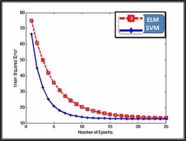
Figure 2: Mean Squared Errors for 10 experiments with step size.

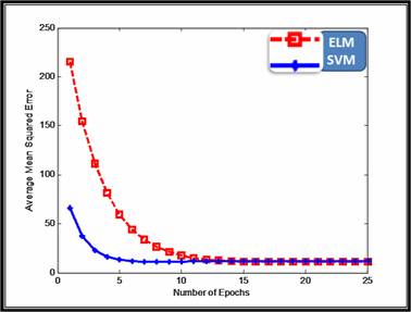
Figure 3: Average Testing MSE for 15 experiments.

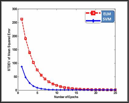
Figure 4: Standard Deviation of Testing MSE for 15 experiments.

The performance of both ELM and SVM versus the most common predictive data mining techniques in statistics and computer science communities in identifying the carbonate lithofacies from well logs were calculated and investigated. We record only the results based on the utilization of SVM, ELM, and ANN for the sake of simplicity. Table 1 shows the percentage of data points which were misclassified using ANN, ELM and SVM for each of the class label. For example, 22.2% of the data points whose true class label is 1 were misclassified as some other class, using ANN.  
  The detailed results are summarized in Table 2 with Figures 5 and 6. From this Table and these Figures, we concluded that both ELM and SVM outperforms the most common existing predictive models, especially, multilayer perceptron feedforward neural networks. The ELM has the smallest computational time with a proper correct classification rate, 84.96%. On the other hand, SVM has the highest correct classification rate, 88.31% with adequate computational time.

Table 1 Testing results: The overall performance with 10-fold cross validations.  

Table 2 Testing results: The overall performance with 10-fold cross validations.

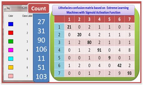
Figure 5: Lithofacies Identifications based on extreme learning machines: Confusion matrix and overall performance.

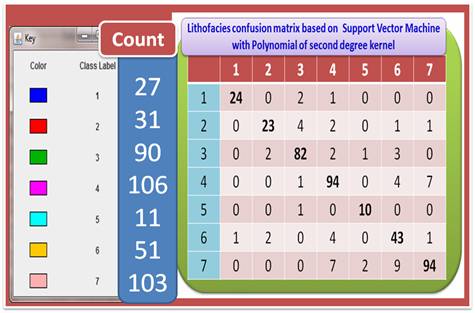
Figure 6: Lithofacies Identifications based on support vector machines: Confusion matrix and overall performance.

Conclusion

In this research, we have investigated both extreme learning machines and support vector machines capabilities in identifying the Litho-Facies from conventional well logs. A general framework is built to handle imprecision and uncertainty in Litho-Facies models and different steps of this framework has been discussed in details. Validation of the framework has been done using some well log data.
Both ELM and SVM outperform the most common existing predictive models, especially, multilayer perceptron feedforward neural networks. In addition, the ELM has the smallest computational time with a proper correct classification rate. On the other hand, SVM has the highest correct classification rate.
The following are some of the possible future work to be accomplished in the field of oil and gas industry along the same research direction, namely: (i) More experiments can be carried out if data is available with uncertain numerical attribute measurements; and (ii) Since ELM and SVM Mode still have some limitations, future work can be focused towards this direction to make the framework more robust.

Acknowledgement

The authors would like to acknowledge the support provided by King Abdulaziz City for Science and Technology (KACST) through the Science & Technology Unit at King Fahd University of Petroleum & Minerals (KFUPM) for funding this work under Project No. 08-OIL82-4 as part of the National Science, Technology and Innovation Plan. We wish to thank MEDai Inc., an Elsevier Company for their support and facilities required for this research.

References

1. Ferraz, I.N.; Garcia, A.C.B.; Litho-Facies recognition hybrid bench, Fifth International Conference on Hybrid Intelligent Systems, 6-9 Nov. 2005.
2. Alain Bonnet and Claude Dahan, Oil-Well Data Interpretation Using Expert System and Pattern Recognition Technique, International Joint Conferences on Artificial Intelligence (IJCAI), 1983.
3. Hinton G. E., “Connectionist learning procedures”. Artificial Intel., 40:185–234, 1989.
4. White H., “Learning in artificial neural networks: A statistical perspective”. Neural Comput., 1:425–464, 1989.
5. Abdulraheem A., El-Sebakhy E., Ahmed M., Vantala A., Raharja I., and G.  Korvin, “Estimation of Permeability From Wireline Logs in a Middle Eastern Carbonate Reservoir Using Fuzzy Logic”.  The 15th SPE Middle East Oil & Gas Show and Conference held in Bahrain International Exhibition Centre, Kingdom of Bahrain, 11–14 March 2007.  SPE 105350. 
6. E. A. El-Sebakhy, Abdulraheem A., Ahmed M., Al-Majed A., Raharja P., Azzedin F., and Sheltami T., “Functional Networks as a Novel Approach for Prediction of Permeability and Porosity in a Carbonate Reservoir”, the 10th Int. Conference on Eng. Applications of NNs  EANN2007,  Thessaloniki, Hellas, Greece. (29-31) August, page(s) 422-433, 2007.
7. Smith, M.; Carmichael, N.; Reid, I.; Bruce, C.; Litho-Facies determination from wire-line log data using a distributed neural network, Proceedings of the Neural Networks for Signal Processing, IEEE Workshop, 30 Sept.-1 Oct. 1991, Pp 483 – 492.
8. Kozhevnikov, D.A.; Lazutkina, N.Ye.; Nuclear geophysics methods - An information kernel of logging data complex interpretation system, Nuclear Science Symposium and Medical Imaging Conference, 1994 IEEE Conference Record, Volume 1,  30 Oct.-5 Nov. 1994, Pp:361 – 366.
9. Hsien-Cheng Chang, David C. Kopaska-Merkel, Hui-Chuan Chen and S. Rocky Durrans, Litho-Facies Identification using multiple adaptive resonance theory neural networks and group decision expert system, Computers & Geosciences Volume 26, 2000, Pages 591-601.
10. Hsien-Cheng Chang, David C. Kopaska-Merkel and Hui-Chuan Chen, Identification of Litho-Facies using Kohonen self-organizing maps, Computers & Geosciences Volume 28, Issue 2, March 2002, Pages 223-229.
11. Ferraz, I.N.; Garcia, A.C.B.; Litho-Facies recognition hybrid bench, Fifth International Conference on Hybrid Intelligent Systems, 6-9 Nov. 2005.
12. Wohlberg, B.; Tartakovsky, D.M.; Guadagnini, A.; Subsurface characterization with support vector machines,
    IEEE Transactions on Geoscience and Remote Sensing, Volume 44,  Issue 1,  Jan. 2006, Pp 47 – 57.
13. Guang-Bin Huang, Qin-Yu Zhu, Chee-Kheong Siew, “Extreme learning machine: Theory and applications”, Neurocomputing 70, 489–501, (2006).
14. Vapnik V., The nature of statistical learning theory, Springer, New York (1995).
15. C. Cortes and V. Vapnik, “Support-vector networks,” Mach. Learn., vol. 20, pp. 273–297, 1995.
16. K.L. Peng, C.H. Wu and Y.J. Goo, The development of a new statistical technique for relating financial information to stock market returns, International Journal of Management 21 (2004) (4), pp. 492–505.
17. Emad A. El-Sebakhy, (2004), “A Fast and Efficient Algorithm for Multi-class Support Vector Machines Classifier”, ICICS2004: 28-30 November. IEEE Computer Society, pages: 397-412.
18. Emad A. El-Sebakhy, Forecasting PVT properties of crude oil systems based on support vector machines modeling scheme. Journal of Petroleum Science and Engineering, Volume 64, Issues 1-4, (2009), Pages 25-34.
19. E. Osuna, R. Freund, and F. Girosi, “Training support vector machines: An application to face detection,” IEEE Conf. Comput. Vis. Pattern Recognition, pp. 130–136, Jan. 1997.
20. D. R. Hush and B. G. Horne, Progress in supervised neural networks: What’s new since lippmann? IEEE Signal Processing Magazine, vol. 10, no. 1, pp. 8–39, January 1993.

AAPG Search and Discovery Article #90105 © 2010 AAPG GEO Middle East Conference & Exhibition, Manama, Bahrain, 7-10 March 2010