![]() Click to view this article in PDF format.
Click to view this article in PDF format.
Mapping Geologic Structure of Basement and Role of Basement in Hydrocarbon Entrapment*
Parker Gay1
Search and Discovery Article #40052 (2002)
*Adapted for online presentation from two articles by the author in AAPG Explorer (November and December, 1999), respectively entitled “Basement Mapping Highly Crucial” and Maps: It’s the Basement’s Fault.” Appreciation is expressed to the author and to M. Ray Thomasson, former Chairman of the AAPG Geophysical Integration Committee, and Larry Nation, AAPG Communications Director, for their support of this online version.
1Applied Geophysics, Salt Lake City; [email protected].
In earlier "Geophysical Corner" articles (AAPG Explorer, May and June, 1997; Search and Discovery, 2001), geophysicist Dale Bird discussed conventional uses of aeromagnetics. This article, on the other hand, deals with new and strikingly different uses of aeromagnetics that are emerging. These new uses are based on a better understanding of basement geology and how it affects the overlying sedimentary section.
First, it is necessary to understand the structural nature of basement, and here I refer to Precambrian metamorphic basement that comprises the major shield areas of the world, such as the Canadian Shield, South American Shield, African Shield, Baltic Shield, etc. Shields are simply the outcrop areas of cratons, or continents, and similar metamorphic terranes are located under all cratonic sedimentary basins.
|
|
Figure Captions
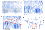
Examples of Basement Structure Figure 1 is a Landsat photograph that covers a portion of the Canadian Shield (NW part) and a portion of the adjacent Ontario sedimentary basin (SE part), where the shield is overlapped by oil-bearing lower Paleozoic strata. The highly fractured nature of basement in outcrop is obvious, but the sedimentary rocks in the basin hide this fracture pattern from view. The basement fractures are reactivated at later times during, or after, deposition of the sedimentary section and create structures and/or sedimentary facies that become oil and gas traps and reservoirs. Thus, the mapping of the fracture pattern under the sedimentary section is of great importance in hydrocarbon exploration. How can this best be accomplished? Neither seismic nor gravity methods can map the basement fracture pattern, although both can map part of it. Subsurface data cannot map the basement in any detail due to the limited number of basement intercepts in most basins. Only magnetics can map the covered basement fault block pattern. Why can magnetics do this? It is because of the rock type changes (resulting in magnetic susceptibility changes) that occur across the basement faults. Figure 2 is a detailed surface geology map of a 30 x 30 mile (50 x 50 km) block of basement on outcrop in Wisconsin. The basement faults (actually shear zones) are shown, and the rock type changes across them are obvious. Shear zones in the basement are one, two, or three kilometers in width, are characterized by crushed and broken rock across the entire width, and are usually steeply dipping. It is these pre-existing zones of weakness that relieve stresses resulting from later tectonic events and/or sedimentary loading. Stresses are not generally relieved by newly formed faults at ±30° to maximum compressive stress, at least not in the last two billion years. Other characteristics of importance:
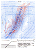
The resulting melange of basement blocks is called the "basement fault block pattern. " Mapping of BasementHow does one go about mapping the basement fault block pattern with magnetics? Figure 3a shows a total intensity aeromagnetic survey on the north flank of the Anadarko Basin, Oklahoma, flown with one-mile spaced east-west flight lines. The sedimentary section is 10,000-12,000 feet thick; the aircraft was approximately 1,000 feet above mean terrain. This map is dominated by a single magnetic high on the west and an elongated low on the east, 16 miles away. It obviously is not mapping the blocks. To bring out the individual blocks it is necessary to residualize the data or to calculate second derivatives. Either will suffice, although some computational techniques are better than others (I prefer profile residuals calculated along flight lines where possible, as shown in Figure 3b). Each of the magnetic highs and lows represents a separate basement block, and the faults (shear zones) occur on the intervening boundaries, or gradients. These faults have been marked with shear zone symbols (red) in Figure 3c; the fault block pattern by itself appears in Figure 3d (blue). A detailed subsurface map of this area yielded only two faults cutting the sedimentary section (shown in red in Figure 3d). They occur precisely along or very close to the mapped basement faults as hypothesized. This is but one example of the correlation of basement shear zones with mapped faults. Since 1982 we have generated hundreds of such cases of correlating faults. Also shown in red in Figure 3d is a structural high mapped using subsurface data at West Campbell Oil Field that falls between basement shear zones. As basement shear zones generally erode “low,” we hypothesize that the West Campbell high is coincident with a basement topographic high and was formed by differential compaction. Compaction anticlines represent another type of basement control important in exploration. Figure 3 is useful in demonstrating another point: Both subsurface faults shown have magnetic lows on their upthrown sides. If structure were the only factor in determining magnetic amplitudes, magnetic highs would occur on the upthrown sides. However, the lithology of the basement is the primary influence on magnetic maps, and structure is a secondary, and sometimes insignificant, factor. Anticlinal Oil Fields Over Basement Faults Figure 4 shows the relationship of an asymmetric fold (Ponca City field, Kay County, Oklahoma, with production to 1993 > 12 million barrels) to an underlying basement fault, shown with shear zone symbols. Pennsylvanian compression reactivated the fault, forcing the west side up along a west-dipping fault to give rise to the overlying fold in Paleozoic strata (see lower part of Figure 4). The fault is "blind", as it does not break through to the level of the folded strata. Figure 5 shows a fault that has broken through to the level of the folded strata in Sage Creek anticline in the Wind River Basin, Wyoming, resulting in a thrust-fold structure. The location of the thrust at basement level is shown by shear zone symbols. This is but one of a chain of several folds in the western Wind River Basin that correlates closely with mapped basement faults. It has a strike length of 70 miles and involves seven separate faults. Four faults are northwest-trending, parallel to the Casper Arch thrust; three are cross-faults that successively offset the northwest-trending faults to the north. We have developed over two dozen examples of asymmetric folds related to basement faults such as those shown in Figures 4 and 5. The cause and effect relationship can be clearly seen. The conclusion is apparent that pre-existing basement faults are reactivated to give rise to the fold-forming faults in the overlying sedimentary section. As noted above, the best (and only) way to map the basement fault pattern in sedimentary basins is with properly processed and interpreted aeromagnetic data. Stratigraphic TrapsI shall try to substantiate the claim that many--and possibly a majority--of oil and gas fields are controlled by basement, with examples of several different types of "purely" stratigraphic traps related to basement faults. Some geologists may concede that the evidence for underlying basement control is convincing. Others will not. I argue that, if a basement fault is in exactly the right location and has exactly the right strike direction relative to a stratigraphic feature of interest, it probably is not coincidental. It must be cause and effect. Oolite Shoal Over Basement Fault Figure 6 shows the location of a southwest Kansas oil field in Pennsylvanian oolitic limestones. The oolite bank was deposited on the probable upthrown side of an underlying basement fault. A nearby fault mapped from seismic data is also shown in red, as are the structural contours on top of the Pennsylvanian limestone. Pennsylvanian Algal Mound Over Basement FaultFigure 7 shows the relationship of a Pennsylvanian algal mound field in Utah to an underlying basement fault. Uplift of the north edge of the tilted basement block under the field could have raised the sea floor to a shallow water environment, allowing the development of the algal mound. Offshore Bars Over Basement Faults Figure 8 shows the relationship of Hartzog Draw Field (that has produced approximately 220 million barrels of oil) in the Powder River Basin, Wyoming, to an interpreted underlying basement fault. Swift and Rice (1984) proposed that the sandstone reservoir in this field and other similar fields in the basin were formed by the winnowing action of bottom currents over sea floor highs. The sea floor high could have resulted from the raising of a basement block edge during late Cretaceous (Laramide) compression. Other nearby fields showing similar one-to-one relationships to magnetically mapped basement faults are:
Fluvial Systems Along Basement FaultsFigure 9 shows the prolific Fiddler Creek Field (in the Powder River Basin), which produces from a lower Cretaceous fluvial sand in the Muddy Formation, as it relates to an underlying interpreted basement fault. Fracturing and jointing along this fault zone would have made the underlying rocks more susceptible to erosion, creating a topographic low along which the river flowed and deposited sands. We have located four other such correlations of fields in the Muddy Formation in this basin with underlying basement faults:
Of related interest, several of the present-day drainages in the basin, such as the Belle Fourche and Little Powder Rivers, follow precisely along basement faults for long stretches. Shoreline Bars along Basement FaultsFigure 10 shows the prolific Echo Springs - Standard Draw - Coal Gulch Late Cretaceous shoreline bar (>l tcf of gas) in Wyoming's Washakie Basin, and its relationship to an interpreted basement fault. Because of the manner in which the sands are stacked, an up-to-the-west fault on the west side of the field is expected (John Horne, personal communication, 1998). It is precisely here that a magnetically mapped basement fault is located. The throw on this fault is minimal, perhaps a few tens of feet, as suggested by comparison to faults controlling deposition in the similar Cardium Formation in the Western Alberta Basin (e.g., Hart and Plint, 1993). This small amount of throw was below the limit of resolution of a 3-D seismic survey carried out over the field's northern part in 1996-97 (Favret and Clawson, 1997). As noted above, the creation of fracture reservoirs is closely related to fault control, but in fracture plays the amount of vertical fault movement can be minimal. We have documented a number of cases where fracture production is coincident with mapped basement faults. In southern Ohio in the Appalachian Basin, for example, a 250% increase in the average gas production in a Clinton-Medina well resulted from drilling on a magnetically defined fracture intersection. Our most compelling fracture correlation has been in the Bakken play of North Dakota, where we obtained production data on 158 horizontal wells and used a computer program to calculate all EUR's in similar fashion. This database was compared to locations of magnetically defined basement faults. Wells drilled in corridors 1.5 miles (2.4 km) wide centered on basement faults yielded 21 percent higher EUR's than those drilled farther away. In the southeast quadrant of the play this figure was 41 percent higher. Many of these wells were drilled parallel or subparallel to basement faults, and at the edges of the corridors. We believe the production figures would have been higher if the wells had been drilled with a knowledge of the locations and strike of the basement faults beforehand. Why? Because eight wells drilled within a 0.75-mile radius of basement fault intersections yielded EUR's 85 percent higher than wells away from intersections. Comments On Other Magnetic Mapping Techniques How do the above processing and interpretational techniques for basement compare to the new "HRAM" methods? "HRAM" stands for "high resolution aeromagnetics," a technique that employs very tight flight line spacing (100-500m) flown at low flight levels (50-150m) and generally displayed as color-coded shade relief maps of total intensity. It is claimed that HRAM can map the traces of faults within the sedimentary section due to magnetite formed along the faults and can locate areas of higher surface diagenetic magnetite content related to micro-seepage. Both of these claims are speculative and controversial. It is also claimed that HRAM can locate pipelines and other cultural features; this is true, but these have questionable value in exploration. For basement mapping there is no technical or computational advantage for the tight flight line spacings and low level flying employed by HRAM. Final StatementThe foregoing examples and figures should demonstrate to exploration managers that the magnetic method, properly applied, is an indispensable tool in almost any exploration program. Magnetics, however, has not been generally used to map basement faults. Instead, the technique has been applied mainly to peripheral problems of lesser importance, such as depth estimation. With the increasing effectiveness of 3-D seismic, magnetics has thus fallen behind in use. ReferencesBird, D., 2001, Interpreting magnetic data, Search and Discovery Article #40022. Clark, S.K., and J.I. Daniels, 1929, Relation between structure and production in the Mervine, Ponca, Blackwell, and South Blackwell oil fields, Kay Cunty, Oklahoma, in Structure of typical American oil fields, v. 1: AAPG special publications, p. 158-175. Favret, P., and S. Clawson, 1997, 3-D reservoir characterization with horizon visualization and coherency/inversion animations, GGRB, Wyoming (abstract): AAPG Bulletin, v. 81, p. 131. Hart, B.S., and A.G. Plint, 1993, Tectonic influence on deposition and erosion in a ramp setting: Upper Cretaceous Cardium Formation, Alberta Foreland Basin: AAPG Bulletin, v.77, p. 2092-2107. Krivanek, C.M., 1981, Bug field, T36S-R25E and R26E, San Juan County, Utah, in Geology of the Paradox basin: RMAG, p. 1-21. LaBerge, G.L.1981, Marathon County area, in 1981 Archean geochemistry field conference; Upper Peninsular and northern Wisconsin, IGCP, Archean Geochemistry Project, U.S. Working Group, United States. Lowman, P.D., Jr., P.J. Whiting, N.M. Short, A.M. Lohmann, and G. Lee, 1992, Fracture patterns on the Canadian Shield; a lineament study with Landsat and orbital radar imagery, in Basement tectonics, v. 1: Proceedings of the Seventh International Conference, p. 139-159. Slamal, B. 1985, Collier Flats field, Comanche County, Kansas, in P.M. Gerlach and T. Hansen, eds., Kansas oil and gas fields, v. 5: Kansas Geological Society, p. 43-52. Swift, D.J.P., and D.D. Rice, 1984, Sand bodies on muddy shelves--a model for sedimentation in the Western Interior seaway, North America, in C.T. Siemers and R.W. Tillman, eds., Ancient shelf sediments: SEPM Special Publication No. 34, p. 43-65. |


 Figure
4. Ponca City Field, Kay County, Oklahoma. This asymmetric, or
compressional, anticline has produced >12 million barrels of oil from
multiple horizons.
Figure
4. Ponca City Field, Kay County, Oklahoma. This asymmetric, or
compressional, anticline has produced >12 million barrels of oil from
multiple horizons.
 Figure
6. Collier Flats Field, Comanche County, Kansas.
Figure
6. Collier Flats Field, Comanche County, Kansas. Figure
7: Bug Field, Paradox Basin, San Juan County, Utah, showing correlation
between a producing Pennsylvanian algal mound and a basement block
boundary.
Figure
7: Bug Field, Paradox Basin, San Juan County, Utah, showing correlation
between a producing Pennsylvanian algal mound and a basement block
boundary. Figure
8. Hartzog Draw Field (Powder River Basin), Campbell County, Wyoming.
Figure
8. Hartzog Draw Field (Powder River Basin), Campbell County, Wyoming.
 Figure
10. Echo Springs - Standard Draw - Coal Gulch Field, Sweetwater Country,
Wyoming, in the Washakie Basin, > 1 tcf of gas.
Figure
10. Echo Springs - Standard Draw - Coal Gulch Field, Sweetwater Country,
Wyoming, in the Washakie Basin, > 1 tcf of gas.