![]() Click
to article in PDF format.
Click
to article in PDF format.
Handbook on Static Pressures*
By
D. E. Powley1
Search and Discovery Article #60007 (2006)
Posted May 1, 2006
*Amoco Production Company Research Department Report F87-G-19, August 3, 1987
1Amoco Production Company, retired, Tulsa, Oklahoma 74136
Introduction
This report was prepared to fulfill the dual objectives of (1) being used as Section 15 in the Amoco training manual “Advanced Formation Evaluation” currently undergoing extensive revisions, and (2) being a report of part of the investigation conducted pursuant to Geological Research Proposal 86-7 “Develop Methods for Estimating Volumes of Sand Bodies and Heights of Hydrocarbon Columns within Overpressured Fluid Compartments.” The format of the report follows the requirements of the Amoco Training Center in Houston. The succession of topics progresses from basic to complex to allow for terminations of training courses anywhere within the text. The report should provide office engineers and operations geologists who are inexperienced in the use of subsurface fluid pressures with a jump-start into semiprofessional level interpretations of static; i.e., nontransient, pressures data. This report will be followed by a companion report which will deal with techniques used mainly by specialists in the interpretation of regional static pressures.
|
uRecognition of abnormal pressures uFigs. 15-13 - 15-20, Table 15-1 uPressures interpretations of water uPressures interpretations of petroleum uInterpretations of fluids within seals
uRecognition of abnormal pressures uFigs. 15-13 - 15-20, Table 15-1 uPressures interpretations of water uPressures interpretations of petroleum uInterpretations of fluids within seals
uRecognition of abnormal pressures uFigs. 15-13 - 15-20, Table 15-1 uPressures interpretations of water uPressures interpretations of petroleum uInterpretations of fluids within seals
uRecognition of abnormal pressures uFigs. 15-13 - 15-20, Table 15-1 uPressures interpretations of water uPressures interpretations of petroleum uInterpretations of fluids within seals
uRecognition of abnormal pressures uFigs. 15-13 - 15-20, Table 15-1 uPressures interpretations of water uPressures interpretations of petroleum uInterpretations of fluids within seals
uRecognition of abnormal pressures uFigs. 15-13 - 15-20, Table 15-1 uPressures interpretations of water uPressures interpretations of petroleum uInterpretations of fluids within seals
uRecognition of abnormal pressures uFigs. 15-13 - 15-20, Table 15-1 uPressures interpretations of water uPressures interpretations of petroleum uInterpretations of fluids within seals
uRecognition of abnormal pressures uFigs. 15-13 - 15-20, Table 15-1 uPressures interpretations of water uPressures interpretations of petroleum uInterpretations of fluids within seals
uRecognition of abnormal pressures uFigs. 15-13 - 15-20, Table 15-1 uPressures interpretations of water uPressures interpretations of petroleum uInterpretations of fluids within seals
uRecognition of abnormal pressures uFigs. 15-13 - 15-20, Table 15-1 uPressures interpretations of water uPressures interpretations of petroleum uInterpretations of fluids within seals
uRecognition of abnormal pressures uFigs. 15-13 - 15-20, Table 15-1 uPressures interpretations of water uPressures interpretations of petroleum uInterpretations of fluids within seals
uRecognition of abnormal pressures uFigs. 15-13 - 15-20, Table 15-1 uPressures interpretations of water uPressures interpretations of petroleum uInterpretations of fluids within seals
uRecognition of abnormal pressures uFigs. 15-13 - 15-20, Table 15-1 uPressures interpretations of water uPressures interpretations of petroleum uInterpretations of fluids within seals
uRecognition of abnormal pressures uFigs. 15-13 - 15-20, Table 15-1 uPressures interpretations of water uPressures interpretations of petroleum uInterpretations of fluids within seals
uRecognition of abnormal pressures uFigs. 15-13 - 15-20, Table 15-1 uPressures interpretations of water uPressures interpretations of petroleum uInterpretations of fluids within seals
uRecognition of abnormal pressures uFigs. 15-13 - 15-20, Table 15-1 uPressures interpretations of water uPressures interpretations of petroleum uInterpretations of fluids within seals
uRecognition of abnormal pressures uFigs. 15-13 - 15-20, Table 15-1 uPressures interpretations of water uPressures interpretations of petroleum uInterpretations of fluids within seals
uRecognition of abnormal pressures uFigs. 15-13 - 15-20, Table 15-1 uPressures interpretations of water uPressures interpretations of petroleum uInterpretations of fluids within seals
uRecognition of abnormal pressures uFigs. 15-13 - 15-20, Table 15-1 uPressures interpretations of water uPressures interpretations of petroleum uInterpretations of fluids within seals
uRecognition of abnormal pressures uFigs. 15-13 - 15-20, Table 15-1 uPressures interpretations of water uPressures interpretations of petroleum uInterpretations of fluids within seals
uRecognition of abnormal pressures uFigs. 15-13 - 15-20, Table 15-1 uPressures interpretations of water uPressures interpretations of petroleum uInterpretations of fluids within seals
uRecognition of abnormal pressures uFigs. 15-13 - 15-20, Table 15-1 uPressures interpretations of water uPressures interpretations of petroleum uInterpretations of fluids within seals
uRecognition of abnormal pressures uFigs. 15-13 - 15-20, Table 15-1 uPressures interpretations of water uPressures interpretations of petroleum uInterpretations of fluids within seals
uRecognition of abnormal pressures uFigs. 15-13 - 15-20, Table 15-1 uPressures interpretations of water uPressures interpretations of petroleum uInterpretations of fluids within seals
uRecognition of abnormal pressures uFigs. 15-13 - 15-20, Table 15-1 uPressures interpretations of water uPressures interpretations of petroleum uInterpretations of fluids within seals
uRecognition of abnormal pressures uFigs. 15-13 - 15-20, Table 15-1 uPressures interpretations of water uPressures interpretations of petroleum uInterpretations of fluids within seals
uRecognition of abnormal pressures uFigs. 15-13 - 15-20, Table 15-1 uPressures interpretations of water uPressures interpretations of petroleum uInterpretations of fluids within seals
uRecognition of abnormal pressures uFigs. 15-13 - 15-20, Table 15-1 uPressures interpretations of water uPressures interpretations of petroleum uInterpretations of fluids within seals
uRecognition of abnormal pressures uFigs. 15-13 - 15-20, Table 15-1 uPressures interpretations of water uPressures interpretations of petroleum uInterpretations of fluids within seals
uRecognition of abnormal pressures uFigs. 15-13 - 15-20, Table 15-1 uPressures interpretations of water uPressures interpretations of petroleum uInterpretations of fluids within seals
uRecognition of abnormal pressures uFigs. 15-13 - 15-20, Table 15-1 uPressures interpretations of water uPressures interpretations of petroleum uInterpretations of fluids within seals
uRecognition of abnormal pressures uFigs. 15-13 - 15-20, Table 15-1 uPressures interpretations of water uPressures interpretations of petroleum uInterpretations of fluids within seals
|
Fluid Pressures - General
Text
Pressure is the force per unit area which fluids (liquids and gases)
exert on the surface of any solid which they contact. Pressure exists at
every point in a fluid at rest. The magnitude of the pressure is
proportional to the In the earth, the datum water surface usually cannot be seen. However, pressure calculations commonly indicate that the rock pores are fluid-filled and interconnected from the top of the free water in the soil down to at least intermediate depths. Inasmuch as the soil water surface is usually only a few inches to a few feet below the topographic surface, it has become common practice to consider the free water surface and the topographic surface to be the same. In marine areas, the free water surface is considered to be mean sea level. The hydrostatic pressure is that caused by the weight of a freestanding fluid column without any external pressure being applied. If any external pressure is applied to any confined static fluid, the pressure at every point within the fluid is increased by the amount of the external pressure. This statement is known as Pascal's Principle, after the French philosopher who first clearly expressed it. An example of a confined static fluid is the fluid below a piston in a closed cylinder. The pressure in the fluid increases as external pressure is applied and returns to normal when the pressure is removed. Within the confined static fluid, the rate of increase in pressure downward; i.e., the interval pressure gradient, is the same with or without an external pressure (Figure 15-3). In
geology, the counterpart to the piston and cylinder walls of
Figure 15-3 are any combination of rock
layers, faults, and interfaces which completely enclose a body of
fluid-bearing rock in a low-permeability envelope. The low-permeability
envelope is usually referred to as a seal. A seal is usually thin with
respect to both thickness and lateral extent of the enclosed rock body.
An abnormally pressured rock body is like a huge bottle (Figure
15-4). It has a thin, essentially impermeable outer seal and an
internal volume which exhibits effective internal hydraulic
communication. The interval rate of increase in pressure with increasing
The Keyes Field in northwestern Oklahoma is illustrative of the case in which the rock matrix at the base of each of the two seals bears the entire weight of the overburden, so the fluid pressures start from zero at these levels. All of the fluid pressures are markedly less than the normal 45+/- psi per 100 feet from the surface, so the pressures in the Keyes Field, except those in the shallow beds above the uppermost seal, are termed underpressures(Figure 15-7). The
Carpathian Basin in Hungary is an example of rock load being partially
borne by the fluids below a seal. The fluid pressures are normal from
the surface down to the base of the Pliocene clastics but are greater
than normal below a thick series of lava flows which separate the
Pliocene clastics from the Miocene clastics. Wells drilled on the
northern shelf penetrate the normally pressured Pliocene clastics, the
seal in the lava flows and the subseal high-pressured Miocene
formations, whereas wells drilled in the southern basin usually
penetrate only normally pressured Pliocene clastics. The interval rate
of pressure increase with Pressures which are less than can be attributed to a freestanding water column to the surface were termed underpressures during the discussion of the Keyes field. Likewise, pressures which are greater than can be attributed to a freestanding water column to the surface are termed overpressures. Underpressures and overpressures together compromise the well-known classification, abnormal pressures (Figure 15-9).
Geology of Abnormal PressuresFigures 15-10 to 15-12
TextIn most
deep basins in the world there is a layered arrangement of at least two
superimposed hydraulic systems (Figure 15-10).
The shallowest hydraulic system can extend to great depths; however, in
many basins it extends from the surface down to about 10,000 feet,
greatest historical The deeper hydraulic systems usually are not basinwide in extent and exhibit abnormal pressures. They generally consist of a layer of individual fluid compartments which are sealed off from each other and from the overlying system. In some basins, mainly in the onshore U.S., there is an even deeper, near normally pressured, noncompartmented section (Figure 15-11). The compartmented layer in those basins generally is in the sequence of rocks which were deposited during the period of most rapid deposition. The underlying noncompartmented layer, where present, usually is in pre-basin shelf deposits and basement rock. The uppermost noncompartmented layer usually is in rocks which were deposited during the slowing rate of deposition in late stage in basin filling. Recognition of the layered arrangement of hydraulic systems generally is quite easy. Only a few widely spaced, well-documented deep wells with several tests run over perforated intervals or several pressure readings from repeat formation testers in scattered wells generally are sufficient to outline the overall arrangement of hydraulic systems in each basin. However, in some young, foreign basins and in the Copper River Basin in Alaska, fluidized rock material, mainly shale, and high pressure water with minor hydrocarbons are being locally ejected upward from subsurface overpressured compartments, through overlying normally pressured rocks and venting at the surface. Mud volcanoes may be built up at the vent sites. The rising, high-pressured mixture may pressure-up any shallow, permeable beds encountered, thereby locally complicating recognition of the layered arrangement of hydraulic systems. The individual compartments in the compartmented layer may be very extensive, as in some of the Rocky Mountains basins, or may be only a few miles across, as in the Gulf Coast Basin. The pressures within the compartments are overpressured or underpressured relative to the pressures in both the shallower and deeper hydraulic systems. The compartmented hydraulic systems in currently sinking basins are almost universally overpressured and are underpressured in many onshore basins undergoing erosion. The principal source of overpressures appears to be thermal expansion of confined fluids and the generation of petroleum during continued sinking and the principal source of underpressures appears to be thermal contraction of confined fluids as buried rocks cool during continued uplift and erosion at the surface. Thus, it appears that the compartments have an amazing longevity as they undergo a continuum from overpressures through normal appearing pressures to underpressures as their host basins progress from deposition, to quiescence, to basin uplift and erosion. Fluid compartments are important in subsurface geology because oil and gas may be trapped in external or internal beds where they abut seals or may be in permeable beds within seals. In those basins with three layers of hydraulic systems, the seal between the middle compartmented layer and the underlying noncompartmented layer usually follows a single stratigraphic horizon. For instance, the basal seal of the compartmented section in the central Powder River Basin appears everywhere to be within the thin Cretaceous Fuson shale. However, in many basins, the top seal of the compartmented layer is more complicated. It (1) tends to follow an irregular sands-over-massive-shale boundary in the Gulf Coast and Niger Delta basins, (2) it is within thin evaporites in many onshore European and southwestern U.S. basins, and (3) occurs as horizontal or gently dipping planes which cut indiscriminately across structures, facies, formations, and geological time horizons in the Alaska North Slope Basin, in the northern Cook Inlet Basin, in the Alberta Basin, in the Anadarko Basin, in the North Sea Basin, and in many Rocky Mountains basins (Figure 15-11). Those top seals which do not follow a specific stratigraphic horizon generally are restricted to clastics dominated sections. The planar-topped, compartmented sections are almost universally in basins which are older than the basins in which the compartmented sections exhibit much top surface irregularity. Thus, it appears that there is some process in nature whereby the top seals of compartments in clastics-dominated sections can smooth themselves over time. The leveling process may be quite rapid because the tops of the two principal fluid compartments in the central North Sea Basin are horizontal over distances in excess of 100 miles despite the recent salt-induced structure development in the area. Planar seals may occur within, as well as on the top of the compartmented layer. For instance, the shallowest seal in the Mill Creek graben in southern Oklahoma is everywhere within the thin Marmaton shale; the next deeper seal is horizontal (-10,400 to -11,500 feet elevation), cuts through many Paleozoic formations across the graben and even extends, at the same elevation, across the adjacent Ardmore Basin. No deeper seals have yet been encountered in wells in the graben or in the Ardmore Basin. Earlier
in this chapter it was pointed out that the individual compartments in
the compartmented layer are like huge bottles with thin bounding seals
and huge fluid-communicating internal volumes. Seals are particularly
annoying to work with because they do not have consistent lithologic
properties other than extremely low across-the-seal permeability. In the
absence of unique lithologic properties, recognition must be
accomplished from indirect evidence, such as well log indicators,
measured pressures in local reservoirs encased in seal rock and often
only from the requirement that they must be there separating reservoirs
which, from measured pressure data, are obviously hydraulically
separated from each other. Seals may have thin internal permeable rock
layers (like bubbles in the glass of glass bottles), which may contain
oil and gas pools. The transition of pressures across the total
thickness of top seals in clastic rocks is linear with increasing In some areas, seals may be recognized by calcite and/or silica mineralization within the seals or in the lower pressured rocks exterior to the seals, probably resultant from dissolved minerals being precipitated as water seeps through the seals. The mineral infill of porosity and fractures may be so readily recognizable that it becomes an identifier of present or past seals. For instance, calcite infill is so ubiquitous within seals and in adjacent beds in southwestern Louisiana that it has been given the name “Al's Cap,” named for Al Boatman, a local geologist, who first publicly drew attention to the phenomenon there. Silica infill may be recognizable on the basis of drastically reduced rates of drilling penetration across a seal. For instance, it took 24 hours to cut a 60-foot core in a silica-enriched seal in chalk in the Shell-Esso 30/6-2 well in the North Sea. Chalk normally cores very rapidly, unless the bit becomes clogged. Top seals in clastics dominated sections range in thickness from 150 feet to over 3000 feet; however, the majority are uniformly near 600 feet. Seals in carbonate-evaporite sections are generally somewhat thinner; in fact, some salt and anhydrite beds as thin as 10 feet form effective seals. An example of the latter is the Devonian Davidson evaporite which, except for a small area in central Saskatchewan, is about 20 feet thick but forms a regional seal over almost the entire extent of the Williston Basin. Lateral seals appear to be generally vertical or very nearly vertical. They range in thickness from less than 1/8 of a mile (within the distance between wells on 10 acre spacing) to about six miles, with the majority being 1/8 of a mile or less in width. They tend to be quite straight, which suggests that they may tend to follow fault trends. There has not been any satisfactory suggested geochemical mechanism which could create impermeable walls over thousands of feet of vertical extent through rocks of many lithologies. Where wells have penetrated lateral seals, the rocks have generally been found to be slightly fractured and the fractures infilled with calcite and/or silica. In a few localities, some of the fractures are locally open and can yield limited oil and gas production. While lateral seals are almost always nearly vertical, continuous planes, there are a few remarkable cases of breaks in seal continuity where individual permeable rock layers extend in hydraulic continuity from a compartment into a neighboring compartment. Those tongues are of particular interest to exploration geologists because they frequently contain oil and gas pools. The
rocks in the internal volumes within the compartments, like the seals,
do not have a unique lithology. The most unique property is the
pervasiveness of fractures observed in cores and indirectly indicated by
the apparent hydraulic continuity; i.e., reservoir to reservoir
continuity of interval pressure- The
fractures in the internal volume are, in a few areas, open enough to
permit commercial-rate extraction of oil and gas even in the absence of
significant matrix porosity and permeability. However, the distribution
of open fractures is generally not uniform enough to allow field
development without a substantial proportion of dry holes unless the
fracture porosity is augmented with matrix porosity and permeability
within the internal volume rocks. The matrix rocks, in different areas,
may exhibit remarkably different porosity values. For instance,
sandstone porosities are in the 20-35% range in the overpressured
Cretaceous Tuscaloosa sandstone reservoir in the False River Field in
Louisiana and are generally much less than 10% in the Paleozoic Goddard
sandstone reservoir in the Fletcher Field in Oklahoma at approximately
the same
Recognition and Indirect Quantification of Abnormal PressuresFigures 15-13 to 15-20, Table 15-1
Text
Overpressures have been known and studied in the Gulf Coast Basin for
many years. Most of the techniques to drill and complete wells safely in
overpressured formations now in use worldwide were developed in the Gulf
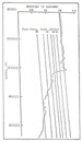
Coast. One of the most significant techniques is the use of well logs to
identify and quantify overpressures. The techniques now in use are
modified from those introduced in a paper presented by Hottman and
Johnson in 1965. They reported the coincidence of high fluid pressures
in sands and lower-than-normal electrical resistivities and acoustic
velocities in adjacent shales (Figure 15-13).
The technique using electrical logs involves an empirical relationship
between the resistivity of shales adjacent to sands with fluids at
normal pressures and the resistivity of shales adjacent to sands with
overpressured fluids. The resistivity values for shales are generally
easy to read on electrical logs. The ratios of the resistivity of the
shales in the normally pressured section to the resistivity of the
shales in the overpressured section are plotted on a ratio comparison
chart which yields a pressure/vertical An
example calculation utilizing Figures 15-15,
15-16, 15-17,
and 15-18 should be made at this point to
ensure that the technique is understood. This example calculation is
somewhat misleading inasmuch as the accuracy obtained is better than
that which can be routinely derived from average quality well logs. The
importance of the foregoing well-log interpretation technique is that it
is possible to construct pressure- A
similar technique, also introduced by Hottman and Johnson (1965),
involving interval sonic velocities derived from sonic logs has been
used widely. The sonic log is fundamentally different than the
resistivity log inasmuch as sonic velocities are affected by fluid
pressures across the whole possible pressure/ It has
been the author's experience that sonic log data are excellent for
picking the tops and bases of both overpressures and underpressures and
tops and bottoms of fluid compartment seals but deriving actual pressure
values is very uncertain because so many lithology effects and rock
porosity effects are involved in the interval velocities in shales. In
some Rocky Mountains and Alaska basins, sonic logs provide the only
reliable log indicators of pressures because the lithology effects and
water salinity effects tend to overwhelm resistivity logs. In west
Texas, sonic logs are difficult to work with because it is hard to find
a “valid” shale. Most shale travel time/ Several
authors have noted that high pressures are frequently accompanied by
higher-than-normal geothermal gradient values. Interval geothermal
gradients in overpressured rocks in which pressure/ Hottman
and Johnson (1965) contended that porosity in shale is abnormally high
relative to its The compaction-pressure technique continues to be applicable in southern Texas where there is a high degree of correlation between the degrees of compaction and pressures. Bob Hix of the Houston Region is the company log analyst most familiar with those techniques; so it would be advisable for geologists and engineers working with overpressured wells in South Texas to contact Bob directly.
Drilling rate is a function of weight on the bit, rotary speed (rpm),
bit type and size, hydraulics, drilling fluid, pore pressures, rock
stresses, and rock characteristics. Under controlled conditions of
constant bit weight, rotary speed, bit type and hydraulics, the drilling
penetration rate in shales decreases uniformly with
Penetration rate should be plotted in 5 to 10 feet increments in
slow-drilling formations or in 30 to 50 feet increments in fast-drilling
intervals. However, plotting such data points should not lag more than
twice the plotted Regardless of how the rate of penetration is recorded, a normal drilling rate trend should be established while drilling shales in normal pressure environments for comparison with faster drilling overpressured shales. Complications can arise due to bit dulling, which may mask any penetration rate change due to overpressures. The penetration rate even may decrease if the rotary torque fluctuates and if the drilling bit action on the bottom of the borehole becomes erratic. Since
it is not always possible and/or feasible to maintain bit weight and
rotary speed constant, an improved method has been developed which
allows plotting of a normalized penetration rate (d-exponent) vs Normalized drilling rate correlations take into account the rotating speed of the bit, the mud weight, the weight on the bit, the bit size, and the actual penetration rate to detect the entrance into an abnormally pressured zone. These relationships are used to determine the weight of mud to hold the fluids in the abnormally pressured zones. The normalized drilling model is defined by:
Log R/(60 N) = Log K + b Log (12 W) /dB (1)
where: R = bit penetration rate, ft/hr
N = rotary speed, rpm
W = bit weight, M lbs
dB = bit diameter, inches
b = bit weight exponent = Log R/(60 NK) Log (12 W)/ dB
K = formation drillability constant
In 1966, Jorden and Shirley proposed simplifying the normalized drilling model to normalize penetration rate data for the effect of changes in weight on bit, rotary speed and bit diameter through the calculation of a “d-exponent” defined by:
d = Log R/(60 N) (2) Log (12 W)/ (1000 dB)
Equation (2) is not a rigorous solution for the “d-exponent” of Equation
(1) in that: (1) the formation drillability constant, K, was assigned a
value of unity, and (2) scaling constants were introduced. Jorden and
Shirley (1966) felt that this simplification would be permissible in the
Gulf Coast area for a single rock type since in this area there are “few
significant variations in rock properties other than variations due to
increased compaction with In 1971, Rehm and McClendon proposed modifying the “d-exponent” to correct for the effect of drilling fluid density changes as well as changes in weight on bit, bit diameter and rotary speed. After an empirical study, Rehm and McClendon computed a “modified d-exponent” using the following equation:
d = d Gpn / Gcd (3)
where: dc = “corrected or modified d-exponent”
d = “d-exponent” defined by Equation (2)
Gpn = normal pore pressure gradient for the area, expressed as equivalent drilling fluid density, lb/gal
Gcd = equivalent drilling fluid circulating density at the bit while drilling, lb/gal
Figure 15-20 is a plot of the calculated
modified “d-exponent” values vs The overlay and “d” equation plot is probably the most accurate method available to on-site drilling engineers to use for the determination of bottomho1e pressure from drilling rates in regions with an abundance of soft shale. It is limited, however, to good data collection facilities and to consistently good drilling practices. Its effective use is also limited to wells which are drilled nearly in balance, particularly in soft shale formations. Artificially induced pore pressures from excess mud weight can be transmitted into the rocks being drilled, making most drilling responses, including drilling exponent, unreliable indicators of country rock pore pressures. The ability to correlate drilling rates with lithology and pore pressures to establish a standard for drilling rates is the key to accurate interpretations. The reader should note that most of the techniques to indirectly quantify pressures in underground reservoirs involve making observations or measurements in adjacent water-shale. This is based on a commonly accepted assumption that there is a close coupling of pressures from reservoir rocks, particularly sandstones, to overlying and underlying shales. The assumption has not been seriously challenged where both the reservoir rock and the adjacent shale are water-filled; however, there have been interpretation problems where the reservoir rock contains oil or gas. Also, there have been a few serious misinterpretations where gas occupies a large part of the porosity in shale. Gassy shale generally exhibits very low interval sonic velocities which can lead to incorrect interpretations that the shale has higher fluid pressures than in the adjacent reservoir rock. Conversely, gassy shale generally exhibits high electrical resistivities which can lead to an incorrect interpretation of lower pressures in the shale than in the adjacent reservoirs. There are many indirect pressure indicators not discussed in this chapter. Table 15-1 lists most of those methods, several of which are specialized techniques applicable to on-site drilling engineers. The material discussed in this chapter is considered to be the minimum level of knowledge about indirect quantification of pressures required by exploitation geologists and office engineers dealing with records of wells drilled into abnormally pressured formations.
Direct Quantification of Pressures
Figures 15-21 to 15-24
TextNone of
the foregoing indirect indicators of abnormal pressures or the pressures
calculated from indirect indicators are as reliable as a few measured
pressures. Until the mid-1970's, the only measured pressures available
in overpressured soft rock sections in most wells were pressures
measured during initial production tests run after the wells were
drilled, cased, and perforated. Open hole drillstem tests have been
routinely run in normally pressured and underpressured firm rock
sections since 1935; however, the reported shut-in pressures tended to
be unreliable because the mud (hydraulic) pressures in the wellbores
usually exceeded formation fluid pressures with possible consequent
distortions in measurements (supercharging) of shut-in formation fluid
pressures prior to opening the tool. The more common problem was that a
measurement of static pressure made after the test was completed was
distorted by drawdown of pressures during testing (Figure
15-21). There is nothing basically wrong with drillstem test tools
or gauges for pressure measurements; the shortcoming is that the usual
purposes for using the tool do not include a serious attempt to measure
the static pressure in the rock interval being investigated. The usual
purposes for using the tool are to determine the type of formation fluid
present, to indicate a short term production rate, to record sufficient
transient (not static) pressures data to provide a basis for estimating
average reservoir permeability within the radius of investigation, and
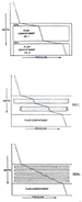
lastly to indicate the extent of wellbore The commercialization of wireline repeatable formation testers in 1974 ushered in a whole new era in well control and well data interpretation. They can record an unlimited number of pressure measurements during a single trip into a wellbore. Two independent formation fluid samples can also be taken on the same trip. Those test tools are reliable, rugged, and very sensitive to minor differences in pressures. They withdraw such a tiny amount of fluid from the formation being tested that drawdown of pressures is not a problem. Pressures measured with repeat formation testers, like pressures measured with drillstem testers, are subject to distortion by supercharging of low permeability rocks by the pressures in the wellbore mud column.
Figure 15-22 portrays the pressures measured
with a wireline repeatable formation tester in a field in the North Sea.
Note that the fluid compartments portrayed in Figures
15-23 and 15-24
have very small but consistent pressure differences from compartment to
compartment. Neither production tests or drillstem tests could have
provided pressure data of similar reliability. The only real limitations
to the use of wireline repeatable formation testers are (1) that the
tester works well only in soft formations, and (2) the tester run must
be preceded by some porosity indicator log, such as an electrical log to
select the depths at which pressures are to be measured. The pressure
values from repeat formation tests should be corrected for temperature
effects on the quartz gauges in the test tools. The corrections are
supplied by the testing contractors. It is suggested that up to 30
pressure measurements be made in water-bearing porous zones over a
Pressures Interpretations of Water in Open Hydraulic Systems
Figures 15-25 to 15-36
TextExploration geologists and well planning engineers have similar problems regarding locating, sorting, and assembling pressure data. Both are required to make interpretations regarding specific sites or specific areas using whatever data are available. Both groups work primarily with water dominated fluids systems. The ensuing discussion, while aimed mainly at well planning engineers, is equally applicable to exploration geologists.
Engineers drawing up the operating specifications for wildcat wells are
frequently faced with the necessity of anticipating static fluid
pressures in underground formations in regions where industry practice
has been to run only about one drillstem test somewhere in each well. At
first glance, it may seem to be impossible to assemble enough data to do
an adequate job of anticipating the pattern of pressures to be
encountered by the planned well. Pressures measured in drillstem tests
have been labeled “unreliable” earlier in this report; however, large
files of unreliable drillstem test data may be used to identify
overpressured and underpressured fluid compartments. Amoco's Well Data I
and Well Data II computer files contain an enormous quantity of
pressures data derived from drillstem tests. When such data from many
wells are plotted onto pressure/
Inasmuch as those data files contain both virgin pressures and pressures
drawndown by production, it seems prudent to attempt to avoid being
misled by local drawndown pressures. Figure
15-25 illustrates the recorded pressures measured at various times
through the life of two fields. Note that the pressures at discovery
(the highest pressures), are significant if a wildcat well is being
planned and the lower pressures have no significance unless the planned
well is to be drilled in, or adjacent to, the field. Figures
15-26, 15-27,
15-28, 15-29,
15-30, 15-31,
and 15-32 illustrate the kinds of fluid
compartment implications which can be derived from critical examination
of large masses of pressure data, even though every data point may be
somewhat unreliable. Pressure/ Duplication of the mud program used in nearby old wells may be sufficient to select an acceptable mud program in a new well; however, mud programs in a few old wells usually cannot be reliably converted into subsurface static pressures in abnormally pressured fluid compartments. Use of mud data from a few old wells is subject to considerable bias ranging from the operator's state of knowledge about pressures at the time the old wells were drilled to how safe-from-blowout the operators of the wells wished to drill their wells.
Figure 15-33 illustrates how large files of
mud density data from well log headers, converted to equivalent
bottomhole pressures, plotted onto pressure/ Some
operators drill wells with slightly underbalanced mud columns to attain
increased drilling penetration rates. Drilling kicks in such wells may
provide accurate indicators of the formation fluids pressure/ The foregoing discussions regarding the use of inaccurate data presumed that the inadequacies are resident in the original data. However, there can be a large error factor introduced by human carelessness all along the line from recording of wellsite data to data introduction into computer files. Transposed numbers; i.e., numbers copied out of sequence, are an ever present menace when making interpretations of subsurface pressures. Figure 15-35 illustrates a typical case of probable transposition of numbers. Transposition of numbers is particularly common in data files which were accumulated from scout check sources, such as Amoco's Well Data I and Well Data II. The interpreter must be willing to ignore suspect data with the consequent hazard that accurate data may be discarded. Some data sources are much more reliable than others. The author has found the data submitted in sworn-to submissions of data in public hearings before the various state and provincial industry regulatory bodies to be a consistently reliable source of data and highly recommends its use where applicable. Figure 15-36 is an example of the data derived from submissions to the Oklahoma Corporation Commission. Note that the data exhibits little scatter, so the inclusion of transposed numbers or guesses instead of real measurements seems to be unlikely.
Pressures Interpretations of Petroleum in Open Hydraulic Systems
Figures 15-37 to 15-68
TextAll prior discussions in this report dealt with water dominated fluids systems. This discussion deals with gas, condensate, and oil-bearing reservoirs in normally pressured rocks and in the internal volumes of fluid compartments (Figure 15-4). The data accuracy requirements when dealing with petroleum are much greater than for water systems, and the zone of interest is generally much thinner when dealing with petroleum.
Petroleum reservoirs almost invariably contain or abut some water; so
the first step in pressure interpretations of petroleum is construction
of a surface to total
Usually, the average water density for a whole basin or basin sector is
accurate enough to establish the slope of a surface to total The
usual purposes of surface to total The last purpose involves the differences in densities of oil, gas, and brines. Figure 15-39 presents a graphical representation of the pressures in a hydrocarbon column vs the pressures to be expected in laterally adjacent water-bearing rocks in the same fluid system. It is important to note that the adjacent water-bearing beds may be normally pressured, overpressured, or underpressured. Oil and gas columns in permeable zones within seals require special handling; so the ensuing discussions will first deal with mixed fluid systems in normally pressured rocks and in the internal volumes of fluid compartments. Please refer to the discussion of fluids within seals (Pressures Interpretations of Fluids within Seals). The
divergence of the oil or gas column pressure/ Operations geologists and office engineers frequently are called upon to estimate the greatest potential vertical height of an oil or gas column over bottom water after oil or gas without water has been recovered in a well test. The updip limit of a hydrocarbon column cannot be determined from pressures data alone; however, the pressure at the top of the petroleum column cannot exceed the local fracture gradient. If the test recovered oil, there is no reliable method to determine if a gas cap is present somewhere above the tested interval. Projecting the vertical height of a hydrocarbon column downward from a test which recovered gas is subject to uncertainties about whether there is a downdip oil leg. If an estimate of a hydrocarbon column below the test is to be made on the assumption that the density of the petroleum recovered in the test is representative of the hydrocarbons throughout the whole column below the tested interval a simple mathematical analysis probably will suffice.
(pp – pw) / (Dw-Dp) = vertical height of the hydrocarbon column in feet
where:
pp is a recorded pressure within the petroleum column stated in psi.
pw
is the regional pressure in water-bearing rocks at the same
Dw is the density of the regional water stated in pounds per square inch per foot.
Dp is the density of the petroleum at reservoir conditions stated in pounds per square inch per foot.
Example: a normally pressured Gulf Coast oil reservoir at 10,000 feet. pp = 4800 psi pw = 4650 psi Dw = 0.465 psi/foot Dp = 0.331 psi/foot (4800 - 4650) / (0.465 - 0.331) = 1112 feet of column below the test
The densities of gas, condensate, and oil are highly sensitive to hydrocarbon composition, temperature, and pressure; so selection of appropriate hydrocarbon density values applicable to reservoir conditions requires conversions from densities measured under surface conditions. The author has found the charts on Figures 15-40, 15-41, 15-42, 15-43, and 15-44 to be satisfactory for reservoirs at shallow to intermediate depths but require extrapolations for deep or high pressure pools. Production Research is currently entering the composition phase characteristics of crude oil, condensate, and gas systems under varying temperatures and pressures into a user friendly computer program called PVT CALC. It will be available in the Regions within a few weeks following completion of this handbook. It is suggested that PVT CALC be used in preference to Figures 15-40 through 15-44 where more precise interpretations are required. If very precise interpretations are required, a sample of the fluids recovered during a well test collected under rather strict well site procedures should be submitted to the Research Center for analysis. The well testing, fluids collection, sample bottling, and shipping procedures will be included in the lab services handbook, currently being revised by Production Research.
Construction of a pressure/
Figure 15-47 illustrates the importance of
accurate determinations of the pressures in the bottom water. The
pressures data shown were in Amoco's files in 1955 when there was an
opportunity to acquire an interest in additional acreage downdip from
the newly discovered Pembina (Cardium) oil pool in Alberta. The
prevailing hydrogeological concept at that time was that the pressures
in any permeable bed are essentially independent of the pressures in
shallower and deeper permeable beds. Therefore, the recorded pressures
in the shallower (Belly River) sands were believed to have no bearing on
the pressures in the oil column in the Cardium sand. The Cardium
pressure exceeded the expected water pressure/
In all cases previously discussed in this report, it was assumed that there is no internal compartmentalization within apparently continuous oil and gas pools. Several of the large pools discovered in recent years, particularly in low permeability sand reservoirs, display evidence of through-going seals dividing large pools into subpools. Determinations of the heights of petroleum columns have been fraught with confusion as interpreters attempted to “push” their data into single petroleum column interpretations. Figure 15-48 displays a subpool (multicompartment) system in an ostensibly continuous large gas pool producing from a single sand. Similar subpools have been noted in the tight gas sand areas in the Rocky Mountains and Alberta and in the downdip Wilcox fields in South Texas.
Figure 15-49 illustrates the pressure/ Nearly all development geologists and office engineers will, at some time, encounter at least one petroleum pool with one or more ponds of formation water located well above the base of the petroleum column. Those occurrences of ponded water; i.e., water which was not forced out when petroleum moved into the trap, were called perched water in old geological and engineering literature. Figure 15-50 illustrates the pressures measured in a gas column in northeastern British Columbia, Canada. One test recovered salty water more than 1000 feet above the deepest gas recovery. The ponded water displays a pressure which is being imposed by the adjacent gas. The water probably occupies a local lens of porosity which was not swept of its water when gas entered the field trap. Bottom water has not yet been encountered in the field. The Recluse to Bell Creek cross-section, shown in Figure 15-51, demonstrates a simple examination of alternative techniques to determine if a continuous static petroleum column extends from one discovery to another, even in the presence of water ponds. The highest oil in the area is at the gas/oil interface in the Bell Creek field, and the lowest oil is at the oil/water interface in the downdip Recluse field. The pressure differential is 2262-1180 = 1082 psi across 3700-430 = 3270 feet, which calculates to 1082 psi/3270 ft = 33.1 psi/100 feet. That indicated density of a static pressure conducting medium corresponds with the density of the reservoir oil in the two fields. Thus, a static continuous oil column from Bell Creek to Recluse is indicated, as illustrated diagrammatically in Figure 15-52. Alternatively, if a pressure/elevation of head conversion is made using either a fresh water or formation water density, the resultant calculated potentiometric surfaces dip strongly downdip, thus requiring a very fast downdip water flow to account for the pressure differential between the fields. Inasmuch as there is no topographically low area within at least a hundred miles to vent water at an approximate +1500 feet elevation, the moving water pressure connector from field to field interpretation, while not conclusively disproved, appears to be very unlikely. The indicated continuous oil column from Bell Creek to Recluse does not necessarily mean that all of the intervening area could be made commercially productive. Wells drilled between the fields have encountered tight reservoir sand or thin oil columns over water. The oil over water tests indicate that there are several water ponds held in place by facies changes in the reservoir sand. There are two small water ponds below the pay within the Bell Creek Field. It seems likely that there are commercial oil fields awaiting discovery between Recluse and Bell Creek and possibly downdip from Recluse. The discovery pressures (Figure 15-53) in three old fields producing from a buried river valley sand reservoir in the Glenrock area of Wyoming clearly indicate that the pressure-transmitting medium from field to field is oil despite two large adjacent areas in which water only was recovered. The diagrammatic map in Figure 15-54 provides a simplistic interpretation of the geographic arrangement of the fields and of the two large water-bearing areas. The pressures in the water ponds indicate that the pressures are controlled by the pressures in the abutting oil. It appears likely that there are at least a few undrilled locations in which oil completions could still be made in the interfields oil column connectors.
Figures 15-55, 15-56,
and 15-57 deal with an area of more
historical significance to Amoco. Figure 15-55
illustrates the pressure/
Figure 15-58, taken from a training slide
used in the petrophysics training program, illustrates how ponds of
water trapped in structural roll-overs between petroleum pools and
sealing faults may exhibit the pressure profiles of the abutting
petroleum. Figure 15-59 portrays a well
offshore Trinidad which encountered water pond in several sands adjacent
to a sealing fault. The pressure/ Up to now, we have been dealing with fluid compartments and normally pressured rocks as if the seals have always been there and have always been intact. There are several recognized compartments in which the bounding seals have been permanently ruptured by erosion or faulting or were breached by natural hydraulic fracturing without subsequent healing. The remaining seal segments apparently are still as impervious to gas, oil, and water as they were when the seals were complete; therefore, recognition of seal segments is very important in petroleum exploration. Pressures within a newly ruptured compartment will progressively change toward equilibrium with the pressures in the external water through fluid leakage into or out of the compartment at the point of rupture. When pressure equilibrium is reached at the elevation of the rupture, there is no pressure differential to move fluids further. If the rupture is large or if the adjacent rocks are very permeable, there may continue to be gravitationally driven fluid movement; i.e., water may trickle into a gas-filled compartment, and the gas may bubble out even if the water and gas pressures are equal. During the in or out movement of fluids, the internal pressure at the elevation of the rupture remains equivalent to the external water pressure. If the rupture is very small or if the adjacent rocks have low permeability, the internal and external fluid systems may laterally coexist for a long time after attainment of pressure equilibrium. If the external pressure is decreased, generally through progressive erosion of cover, the fluids within the compartment will seep out to maintain pressure equilibrium. For illustrative purposes, three positions of pressure-equalizing leaks in a seal bounding a fluid compartment (Figure 15-60) will be discussed. The giant Medrano oil and gas pool on the Cement anticline in Oklahoma occupies an underpressured fluid compartment which leaks at its updip terminus into adjacent normally pressured rocks (Leak A, Figure 15-60). The gas pressure at the updip end of the pool coincides with the adjacent normal pressures (Figure 15-61). The pool probably has leaked as erosion has progressively removed cover, and thereby reduced the external normal pressures. Note that the compartment is normally pressured at its updip terminus, but because gas and oil are less dense than the external water, the pool is underpressured relative to the external water in its full downdip extent. The leakage plume over this field has been extensively used by promoters of geological and geophysical techniques which sense the chemical changes in rocks due to the continued presence of seepage gas. The
giant Milk River gas field in Alberta fills an underpressured fluid
compartment which, like the Medrano pool, is pressure equalized near its
updip terminus with exterior fluids (Leak A,
Figure 15-60). There is some uncertainty about whether the leak is
into normally pressured updip rocks to the south or into a near normally
pressured fluid compartment to the west (Figure
15-62). The pressure/ There
are several gas-filled fluid compartments with updip pressure
equalization into water-filled fluid compartments in the deep basin area
of Alberta. Figures 15-63 and
15-64 show two of those pressure/ Figures
15-65 and 15-66
take another look at the Bough “C” compartment within a compartment
previously shown (Figures 15-55,
15-56, and 15-57).
The pressure/
Figure 15-67 illustrates the pressure/
Operation geologists should become familiar with pressure/ Pressures Interpretations of Fluids within Seals
Figures 15-69 to 15-80
TextEarlier in this report, a fluid compartment was described as having “a thin, essentially impermeable outer seal and an internal volume which exhibits effective hydraulic communication.” An analogy was made between a fluid compartment and a buried bottle. The analogy provides an adequate description of the hydraulic conditions within the internal volumes of fluid compartments, and it is functionally correct regarding seals, but it is somewhat misleading regarding the internal structure of seals. Seals, like the glass in bottles, are essentially impermeable across their total thickness but, unlike glass, may exhibit a high order of internal directional permeability parallel to their outer surfaces. Therefore, a fluid compartment may be like a buried bottle which was constructed of some laminated material rather than being like a buried glass bottle. Figure 15-69 is a restatement of Figure 15-4 but portrays a fuller description of the seal. Several
figures used earlier in this report depicted pressure/ Figure 15-71 carries the reader downward across the page through a progression from two superimposed ordinary fluid compartments through a single fluid compartment with an extra thick top seal which has thick internal permeable layers to an ordinary fluid compartment with a top seal which consists of a layered sequence of microcompartments. The figure is introduced to support the author's contention that many seals, particularly in clastic rocks, seems to be a stacked assemblage of many very thin, but widespread, microcompartments. The individual microseals bounding the microcompartments may be discrete depositional rock layers, like turbidite shale beds, or may be paper-thin microstylolitization zones or mineral-filled zones which cut across the depositional layers. The middle diagram shown on Figure 15-71 portrays an arrangement which is rather rare in the United States but is common in a few foreign countries, particularly in Trinidad. Most of the commercial oil pays there are in a few thick sands in the top seal of a very widespread fluid compartment which extends from onshore eastern Venezuela, across the Gulf of Paria, across the island of Trinidad, to the offshore area east of southern Trinidad. Figure 15-72 shows a U.S. example, in this case, with a single thick, water-loaded sand in the top seal.
Figure 15-73 is an example of the diagram at
the bottom of the page in Figure 15-71.
There are several thin, but very extensive, permeable layers in a
strata-bound top seal. The pressures shown on
Figure 15-73 are from a single site. Figure
15-74 shows the pressures in the same permeable layers along a
traverse from six miles updip to six miles downdip from the site shown
in Figure 15-73. Note that each permeable
layer exhibits internal hydraulic continuity, but each permeable layer
is hydraulically isolated from overlying and underlying permeable
layers. The pressures, from permeable layer to permeable layer, exhibit
a straight line rate of change with increasing
Figure 15-75 shows an early recognition of
the pressures-with-
Figure 15-76 portrays pressures measured in
an old well in a tight gas sand area in Wyoming. The pressures from sand
to sand in the top seal of the large fluid compartment there follow a
straight-line rate of change with increasing
Figure 15-77 portrays a similar linear
increase of pressure with increasing
Figure 15-78 is a pressure
Figure 15-79 portrays the pressure/ Figure 15-80 portrays static pressures along a traverse of fields in a single formation. The traverse extends across a lateral seal between a normally pressured area and an underpressured fluid compartment. The profile is the same as one which would be obtained if it were possible to drill a westerly slanting wellbore staying in the single formation. The lateral seal appears to exhibit a linear rate of pressure change across the seal so lateral seals and top seals may be similar in that regard.
FinaleThe level of skills advanced in this report is sufficient for most day-to-day interpretations of local static pressures in underground formations by operations geologists and office engineers. This report will be supplemented with a later report which will advance into more involved techniques of interpretations of static pressures appropriate to specialists in regional pressure studies.
References and Suggested Reading Alliquander, O., 1973, High pressures, temperatures plague deep drilling in Hungary: Oil and Gas Journal, v. 71, no. 21 (May 21), p. 97-100. Bradley, J.S., 1975, Abnormal formation pressure: AAPG Bulletin, v. 59, p. 957-973. Bradley, J.S., 1976, Abnormal formation pressure: Reply: AAPG Bulletin, v. 60, p. 1127-1128. California Division of Oil and Gas, 1973, California oil and gas fields: Volume I, North and east central California: Sacramento, California. Daines, S.R., 1982, Prediction of fracture pressure for wildcat wells: Journal Petroleum Technology, v. 34, p. 863-874. Debrandes, R., and J. Gauldron, 1987, In situ rock-wettability determination with formation pressure data (in press): SPWLA. Erdle, J.C., 1987, How to get more for your money from drill stem tests: Petroleum Engineers International, v. 59, p. 51-54. Gunter, J.M., and C.V., 1987, Improved use of wireline testers for reservoir evaluation: Journal Petroleum Technology, v. 39, p. 635-644. Higgs, N.G., and J.S. Bradley, 1984, Stress state and fracture development during sedimentary burial from theory and microstructural finite element models: Amoco Geological Research Report F84-G-18. Hottman, C.E., and R.K. Johnson, 1965, Estimation of formation pressures from log-derived properties: Journal Petroleum Technology, v. 17, p. 717-720. Jorden, J.R., and O.J. Shirley, 1966, Application of drilling performance data to overpressure detection: Journal Petroleum Technology, v. 18, p. 1387-1394. Guerrero, E.T., 1966, How to find bottom hole pressure from gas well surface-pressure measurement: Oil and Gas Jounral, November 21, p. 175-176. Moses P.L., 1986, Engineering applications of phase behavior of crude oil and condensate systems: Journal Petroleum Technology, v. 38, p. 715-723. Moses, P.L., 1987, Author’s reply: Journal Petroleum Technology, v. 39, p. 235. Narr, W., and J.B. Currie, 1982, Origin of fracture porosity – example from Altamont Field, Utah: AAPG Bulletin, v. 66, p. 1231-1247. Be careful with this publication. It contains a few errors in mathematics, which lead to an incorrect formula for lateral effective stress under conditions of zero lateral strain. Phelps, G.D., G. Stewart, and J.M. Peden, 1984, The effect of filtrate invasion and formation wettability on repeat formation tester measurements: SPE paper 12962, European Petroleum Conference, London, October 1984. Podio, A.L., S.G. Weeks, and J.N. McCoy, 1984, Low cost wellsite determination of bottomhole pressure from acoustic surveys in high pressure wells: Paper 13,254, SPE Meeting, Houston, September, 1984. Powley, D.E., 1982, The relationship of shale compaction to oil and gas pools in the Gulf Coast Basin: Amoco Geological Research Report F82-G-23. Powley, D.E., 1983, Subsurface fluid compartments: Amoco Geological Research Report F83-G-23. Powley, D.E., 1985, Subsurface temperatures: Amoco Geological Research Report F85-G-5. Rehm, B., and R. McClendon, 1971, Measurement of formation pressure from drilling data: Paper 3601, SPE Meeting, New Orleans, October, 1971, 11 p. Rogers, L., 1966, Shale-density log helps detect overpressures: Oil and Gas Journal, September, p. 126-130. Stuart C.A., 1970, Geopressures: unpublished Shell Oil Company report. Weagant, F.E., 1972, Grimes gas field, Sacramento Valley, California, in R. E. King, ed., Stratigraphic oil and gas fields: AAPG Memoir 16, p. 428-439. |