![]() Click to view page images in PDF format.
Click to view page images in PDF format.
Use of Georeferenced Maps in Exploration
By
Jingyao Gong1 and Larry D. Gerken2
Search and Discovery Article #40039 (2002)
1AAPG, Tulsa, Ok 74101 ([email protected])
2Newfield Exploration Mid-Continent, Tulsa, OK 74102 ([email protected])
Spatial information, which is the core of data essential to petroleum geoscientists, now can be efficiently arranged and managed by use of geographic information system (GIS), such as ESRI’s ArcView and ERDAS’ Imagine. One of the functions of GIS software is to georeference maps, and thereby allow direct comparison of a suite of maps with different scales and projection. Once maps are scanned, or vectorized, and georeferenced, they are easily arranged in a desired order for viewing and analysis.
|
|
Maps are generally scanned with resolution of 300 dpi and are saved in tif format. The scanned map is opened in the “View” window of ERDAS Imagine in order to perform the following: 1. Go to the “Raster” menu and choose “Geometric corrections”; a dialogue box of “Set Geometric Model” opens. 2. Choose “Polynomial” and click OK; the “Polynomial Model Properties” window opens; the scanned map is to be matched to its spatially corresponding points on a reference map, one that is in digital and geographic coordinate system. A “polynomial order” of 3 is satisfactory in most cases. After ”Close” is clicked, the GCP Tool Reference Setup window opens. 3. Choose “Vector Layer” option and click “OK” button. 4. A selection window is opened for users to select a vectorized map as a reference. Themes from ESRI data, such as boundaries of counties or states, are commonly used. After the reference map is selected, it is shown on a second view window that is automatically opened after the selection. 5. Find and click the corresponding points in pairs in the two views, such as the marks of latitude/longitude, if they are present, selected geographic boundaries, etc. on the scanned map. After 10 pairs are selected, go to step 6. 6. Click on the Resample icon in the “Geo 7. Open a blank project in ArcView and add the newly generated map to a view. Technically, this tif map can be used for overlay comparisons, but the defaulted black background of the edge of the map is not pleasant. In order to convert the edge’s color from black to white, use a free extension from ESRI website called “quick and dirty georeferencing.” First, turn on the extension and click on the associated “Write World File” icon to write tifw file for the map. Delete the map from the view. Afterwards, open the map using Adobe Photoshop and delete black background from the edge. It should be noted that the size of the map cannot be changed; otherwise the tifw file is invalid and the map is no longer georeferenced. However, color and text can be edited. An ERDAS-generated tif map has three files; one with .aux extension, one with .rrd extension and the other one with .tif extension. If this type of map is edited in Adobe Photoshop, the special information is absent, and the edited map is not georeferenced. This is the reason why we use software to write a tifw file before the color of a georeferenced map is edited because a tifw file can still recognize the edited map. Once the tifw file is written, the .aux and .rrd files can be deleted. Presented herein is an atlas of selected georeferenced maps of the Middle East derived from AAPG publications. The vectorized maps of Sedimentary Provinces of the World (St. John, Bally, and Klemme, 1984) and fields of the Arabian Plate (Beydoun, 1991) are the bases for the following georeferenced maps: 1. Structure map of Arabian Plate 2. Map of Upper Jurassic source rocks, Arabian Plate 3.
4. Structure map of part of United Arab Emirates (U.A.E.) 5. Structure and isopach maps of Bu Hasa oil field Two databases and illustrations of Bu Hasa features are linked to the structure map of the field.
Figures 1, 2, 3, and 4 show several aspects of the rich hydrocarbon Arabian province--its areal extent, fields, foredeep nature, and the extent and thickness of one of the important sequences of source rocks. The gravity map in Figure 5 extends from the eastern edge of the Zagros foldbelt of southern Iran to U.A.E.; the area includes two gravity-anomaly highs, represented by the Qatar Arch and Marazouk-Dhafra trend, which contain draping folds Bushara (1995) hosting giant fields, such as North field, the world’s largest gas field. Bu Hasa Field, United Arab Emirates U.A.E. on the eastern shelf of the Arabian platform contains northeast-southwest folds at the Cretaceous Thamama level (Figure 6). Major fields are present on two prominent structure-highs (Shah-Asab on the east and Huwaila - Bu Hasa axis on the west. Bu Hasa field (Figure 7) is an north-trending anticline, about 22 mi (35 km) long. The anticline, shaped as a tear drop, tapers in width to the south. The structural relief of about 800 ft (250 m) and an areal closure is about 205 mi2 (535 km2) at the top of the Cretaceous Shuaiba carbonate (Alsharhan, 1993). The multiple pays are Upper Cretaceous limestones. Its estimated reserves, as of 1993, was 20 billion bbl of oil. The isopach map of the Shuaiba Formation (Figure 8) shows that the thickest part of the is about 2 to 3 mi (1.2 to 2 km) wide and trends northwest-southeast for more than 14mi (9 km) across the structural crest. Variations in thickness are due to the changes of depositional environments and erosion. ArcView® can link a feature (oil/gas field, fault, anticline, well, seismic line, etc.) on a map to different kinds of data, such as images and databases. Figure 9 shows that Bu Hasa field is linked to three databases. The first one is the burial history case-study, with nine different properties, in Microsoft Excel format. The second one, also in Excel, is the comprehensive database of field parameters. The third data consists of images of illustrations of field features. Alsharhan, A.S., 1993, Bu Hasa Field--United Arab Emirates, Rub al Khali Basin, Abu Dhabi in AAPG Treatise: Structural Traps VIII, p. 99-127. Alexander, R. G., 1986, California and Saudi Arabia Geologic Contrasts in AAPG Memoir 40: Future Petroleum Provinces of the World, p. 291 –315 Beydoun, Z. R., 1991, The Arabian Plate Hydrocarbon Geology and Potential--A Plate Tectonic Approach: AAPG Studies in Geology No. 33, 77p. Bushara, Mohamed N., 1995, Subsurface Structure of the Eastern edge of the Zagros Basin as Inferred from Gravity and Satellite data: AAPG Bulletin, p. 1259-1273. St. John, Bill, A.W. Bally, and H.D. Klemme, 1984, Sedimentary Provinces of the World--Hydrocarbon Productive and Nonproductive: map and booklet: AAPG. |
 Figure 1. Vectorized map of sedimentary provinces of Middle East and
Europe, along with parts of Asia and Africa (from map of St. John, Bally,
and Klemme, 1984), with productivity or potential shown by color (red or
pink with giant field(s), green with subgiant field(s), yellow
nonproductive).
Figure 1. Vectorized map of sedimentary provinces of Middle East and
Europe, along with parts of Asia and Africa (from map of St. John, Bally,
and Klemme, 1984), with productivity or potential shown by color (red or
pink with giant field(s), green with subgiant field(s), yellow
nonproductive). Figure
2. Vectorized map of oil and gas fields of the Arabian Plate, with
outcrops of basement rocks and ophiolites (from Beydoun, 1991), as overlay
to map of sedimentary provinces. Click on inset map for enlargement.
Figure
2. Vectorized map of oil and gas fields of the Arabian Plate, with
outcrops of basement rocks and ophiolites (from Beydoun, 1991), as overlay
to map of sedimentary provinces. Click on inset map for enlargement. Figure
3. Georeferenced structure map (base of Mesozoic) of the Arabian Plate
(Alexander, 1986), as overlay to map of sedimentary provinces. Click on
inset map for enlargement.
Figure
3. Georeferenced structure map (base of Mesozoic) of the Arabian Plate
(Alexander, 1986), as overlay to map of sedimentary provinces. Click on
inset map for enlargement. Figure
4. Georeferenced map of Upper Jurassic source rocks in Arabian Plate
(Alexander, 1986), as overlay to map of sedimentary provinces. Click on
inset map for enlargement.
Figure
4. Georeferenced map of Upper Jurassic source rocks in Arabian Plate
(Alexander, 1986), as overlay to map of sedimentary provinces. Click on
inset map for enlargement. Figure
5. Georeferenced
Figure
5. Georeferenced  Figure
6. Georeferenced structure map, Shuaiba Formation, in part of U.A.E.
(Alsharhan,
1993), as inset to oil and gas map. Click on inset map for enlargement.
Figure
6. Georeferenced structure map, Shuaiba Formation, in part of U.A.E.
(Alsharhan,
1993), as inset to oil and gas map. Click on inset map for enlargement. Figure
7. Georeferenced structure map of Bu Hasa oil field (Alsharhan, 1993), as
inset to structure map of U.A.E. Click on inset map for enlargement.
Figure
7. Georeferenced structure map of Bu Hasa oil field (Alsharhan, 1993), as
inset to structure map of U.A.E. Click on inset map for enlargement.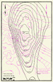 Figure
8. Georeferenced isopach map of Cretaceous Shuaiba Formation, Bu Hasa
field (Alsharhan, 1993), as an overlay to structure map.
Figure
8. Georeferenced isopach map of Cretaceous Shuaiba Formation, Bu Hasa
field (Alsharhan, 1993), as an overlay to structure map. Figure 9. Databases and illustrations of Bu Hasa features, linked to
structure map of U.A.E. (Alsharhan, 1993). Database for Burial History
prepared by M.K. Horn.. Click on burial history plot to
view database in Excel; click on database of field parameters to view it
in Excel; click on illustration for view in PDF.
Figure 9. Databases and illustrations of Bu Hasa features, linked to
structure map of U.A.E. (Alsharhan, 1993). Database for Burial History
prepared by M.K. Horn.. Click on burial history plot to
view database in Excel; click on database of field parameters to view it
in Excel; click on illustration for view in PDF.