Inversion - Interpreting the Deformation Path - Why Does it Matter?*
By
A.D. Gibbs1
Search and Discovery Article # 40034 (2001)
*Adapted for online presentation from poster session by the author at the AAPG Convention, Denver, CO, June, 2001.
1Midland Valley Exploration Ltd, Glasgow, UK. (www.mve.com) ([email protected])
* Editorial Note: This article, which is highly graphic (or visual) in design, is presented as: (1) three posters, with (a) each represented in JPG by a small, low-resolution image map of the original; each illustration or section of text on each poster is accessible for viewing at screen scale (higher resolution) by locating the cursor over the part of interest before clicking; and (b) each represented by a PDF image, which contains the usual enlargement capabilities; and (2) searchable HTML text with figure captions linked to corresponding illustrations with descriptions.
Users without high-speed internet access to this article may experience significant delay in downloading some illustrations due to their sizes.
First Poster
Second Poster
Third Poster
Fourth Poster
Fifth Poster
Most models for inversion focus on understanding the 2D structural development of extension then compression, or occasionally compression then extension. Coupled with this are broad based models that account for the stacking of depositional and erosional packages. These are driven directly by the structural inversion. Inversion is dominantly a 3D process, whether it is driven by the extension - compression cycle, transtension or halokinetic movement. When modeled in 3D it becomes apparent that the 2D cross-sectional view under plays the importance of these systems. Many key commercial basins in Europe and elsewhere contain, or are dominated by, long lived inversion components. Therefore an understanding of the effect of these evolving geometries should be a vital concern. This poster illustrates, through a variety of inversion situations, some key influences on stratigraphy, hydrocarbon systems, and structural control of the deformation path. Key examples are illustrated by some simple 3D models. These highlight the impact of the inversion cycle but in particular the commercial impact of these situations is emphasized.
|
uInversion over complex faults
uInversion over complex faults
uInversion over complex faults
uInversion over complex faults
uInversion over complex faults
uInversion over complex faults
uInversion over complex faults
uInversion over complex faults
|
Click here for sequence of cross sections.
Inversion is defined as occurring when the tectonic regime moves from extension to compression or from subsidence to uplift (Figure 1.1). Some authors have distinguished between positive and negative inversions where a positive inversion ends with a shortening or uplift cycle and a negative with extension and subsidence. These concepts are derived from 2D interpretations of regional systems where a change in regional stress can be demonstrated or inferred. Figure 1.2 is a cartoon of an inverted extension fault. Depocentres in synfault sequences are inverted, leading to a classic pattern of growth wedges controlled by fault bends. Fold hinges and onlap/offlap geometries are pinned to fault bends in the footwall unless modified by footwall deformation. Inversion also occurs without changes to regional tectonic stresses particularly where salt movement imposes differential uplift and subsidence (Figure 1.3). Again this leads to stacked and offset patterns of depocentres. As with fault related inversion, the sequence and evolution of salt movement and sedimentation can be understood through sequential 2D restoration. These 2D cases represent very simple strain histories and the resulting geometries can be readily modeled in 2D. However, in many areas a 2D analysis can be misleading. In addition, the assumption that inversion is caused either by change in regional stress or by halokinesis is a further oversimplification. In many cases oblique faulting, salt displacement and regional changes are combined resulting in mixed inversion and non-inversion styles. Figure 1.4 shows lateral salt migration and faulting with depocentre migration and inversion of accommodation space.
Click here for sequence of A, B, and C.
Click here for sequence of A and B.
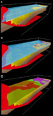
Dip slip inversion in 3D provides significant lateral changes along strike. Modelling demonstrates the importance of modelling the strike component of the system as well as the dip component. The model in Figures 2.1, 2.2, and 2.3 is a 3D equivalent of the simple cartoon shown in Figure 1.2. Even small strike changes in the controlling fault introduce significant variation to map geometry and volume distributions. The object of this modelling is to identify the relationship of depositional packages to fault geometry (architecture) and inversion. During extension (Figure 2.2A, 2.2B, 2.2C), fault geometry controls development of accommodation space. Ray tracing on the developing highs and lows allows sediment transfer systems to the depocentres to be identified. Identifying the sediment catchment areas and depocentre lows provides the geometric framework to interpret the 3D distribution of sediments and aids the production of gross depositional environment maps. In the model, sand fairway (shown in brown, Figure 2.2C) is realized, running oblique to the basin margin. Dip slip inversion is realised in the model in two stages (Figure 2.3A-2.3B). In the first stage (Figure 2.3A), the pre-extension phases are not completely inverted. The cross basin influence of the change in the strike of the fault is seen superimposed above the position of the sand fairway of the earlier stage in the model. As shortening continues all of the depocentres become inverted (Figure 2.3B). With this model using only dip-slip extension followed by inversion, each dip section will be similar. Minor changes along strike combine to produce significant cross-basin or cross-structure elements in the sediment system as well as the structural culminations.
Inversion Over More Complex Faults Click here for sequence of Figure 3.1A and B.
Click here for sequence of Figures 4.1A and 4.2A.
Changes to fault geometry in 3D results in additional complexity in the inverted system. In Figure 3.1 the boundary fault has been modelled with a hard linked transfer. Inversion produces significant offset in structure along the basin. Positioning of the transfer or relay relative to the slip direction effects the separation of depocentres (dark blue) both in the extension and contraction phases (Figure 3.2). Inverting on both the extension and the lateral fault component generates tight inversion structures which place previous synclines in anticlinal positions. Using the same model the effect of changing slip direction during inversion is seen in Figure 3.3. Basin parallel structures become much more segmented and lateral ramps, or relays in the earlier extension system rapidly become dominant in controlling architecture. Amplitude of the inversion folds and rate of growth is controlled by the direction and obliquity of slip. Offsets in the main fault locate the position of transpressional and transtensional components even where the inversion direction is close to the extensional slip (Figure 3.4). Extension on oblique transfer controls sediment catchment areas and accommodation space development. In this model (Figure 4.1), accommodation space may be widely separated with different sediment catchment areas and sediment transfer routes. As the basin inverts, the highs may evolve in positions which are starved of the target sediments. The 3D architecture of the sediment packages during inversion provides different traps, migration fairways, and catchment areas with time. The model (Figure 4.2) shows two time stages (red and blue traps, with hydrocarbon migration pathways yellow and pale blue, respectively) superimposed in the same model. This shows changes in trap geometry, area, and volume, and catchment has changed. Structural highs migrate from yellow to blue position during inversion (Figure 4.2C).
Click here for sequence of Figure 5.1B and C.
2D models assume that salt is drawn and remains within the section; i. e., flow is radial into a dome or salt wall. This model from onshore Germany (Figure 5.1) was used to develop constraints on these assumptions in 3D. The area is composed of two downbuilt diapirs with cross section geometry similar to those shown in Figure 1.3. 3D balanced and restored models for the top salt are shown at two time stages (Figure 5.1B, C). These models show the salt catchment areas and flowage pathways for the salt at each of these time steps. Different coloured areas represent flow packages within the salt. Between the two stages the pattern of catchment areas changes with capture of the cells as the domes grow. As the salt flow pattern changes, there are time equivalent changes in the sediment accommodation space, and inversion occurs as one cell captures or migrates into the zone of influence of another through time.
Baldschuhn, R., U .Frisch, and F. Kockel, 1996, Section 37, in Tectonic Atlas of NW Germany: BGR, Hannover. The author wishes to thank the numerous colleagues and clients who have contributed to the development of this approach. The salt data is from Digitaler Geotektonischer Atlas von Nordwestdeutschland with analysis by Midland Valley. Stephen Calvert assisted in preparing the poster. |


 Figure
2.2. Cross-section panel shows simple listric growth wedge.
Figure
2.2. Cross-section panel shows simple listric growth wedge.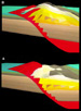 Figure
2.3. Two stages of dip slip inversion. A. Before complete inversion of
pre-extension phases. B. Depocentres inverted.
Figure
2.3. Two stages of dip slip inversion. A. Before complete inversion of
pre-extension phases. B. Depocentres inverted.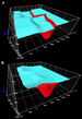 Figure 3.1. Boundary fault with hard linked transfer with
reference surface in extension (A) and after inversion (B).
Figure 3.1. Boundary fault with hard linked transfer with
reference surface in extension (A) and after inversion (B). Figure 3.2. Position of transfer effects the separation of
depocenters in extension (A) and contraction (B).
Figure 3.2. Position of transfer effects the separation of
depocenters in extension (A) and contraction (B). Figure 3.3. Same model as in
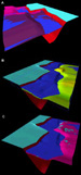 Figure 4.1. Control of sediment catchment areas and
accommodation space by extension on oblique transfer (A). B, C. Positions of
highs evolve as basin inverts.
Figure 4.1. Control of sediment catchment areas and
accommodation space by extension on oblique transfer (A). B, C. Positions of
highs evolve as basin inverts.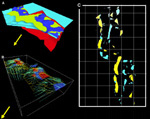 Figure 4.2. Different traps, migration fairways, and
catchment areas form with time during inversion. A. Model after inversion, with
same orientation as in Figure 4.1A. B. Two time stages for traps (red and blue)
and for hydrocarbon migration (yellow and pale blue). C. Map of highs, which
during inversion migrate from yellow to blue position.
Figure 4.2. Different traps, migration fairways, and
catchment areas form with time during inversion. A. Model after inversion, with
same orientation as in Figure 4.1A. B. Two time stages for traps (red and blue)
and for hydrocarbon migration (yellow and pale blue). C. Map of highs, which
during inversion migrate from yellow to blue position.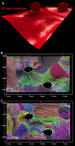 Figure
5.1. 3D salt inversion. a. Diagram of diapirs and top salt. B,C. Balanced and
restored models of salt inversion. Flow packages represented by different
coloured areas.
Figure
5.1. 3D salt inversion. a. Diagram of diapirs and top salt. B,C. Balanced and
restored models of salt inversion. Flow packages represented by different
coloured areas.