Figure 1—Location map of study area, northern Green
Canyon and Ewing Bank, northern Gulf of Mexico.
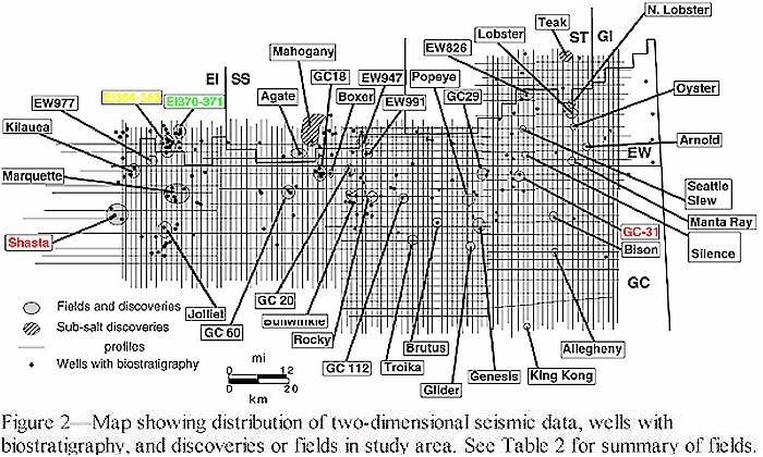
Figure 2—Map showing distribution of
two-dimensional seismic data, wells with biostratigraphy, and discoveries or fields in
study area. See Table 2 for summary of fields.
Figure 3(see animation of
Figures 3, 17, and 18)—Structure contour map on top salt or equivalent salt weld
(contour interval = 1.0 s two-way traveltime). The area is divided into salt bodies
(shallower than 3.0 s two-way traveltime), thin salt (deeper than 3.0 s two-way
traveltime), and salt welds (salt generally less than 100 ms in thickness). The map also
shows areas where shallow salt overhangs deeper levels, and faults that arc around the
lows. A–K indicate the locations of restored seismic profiles; locations of other
Figure are also shown. Map modified from Rowan (1995).
Figure 4(see animation)—Green
Canyon/Ewing Bank portion of megaregional cross section and sequential restorations (1:1
scale):
(A) present-day geometry; (B) 3.0 Ma restoration;
(C) 5.5 Ma restoration;
(D) 8.8 Ma restoration;
(E) 10.5 Ma restoration;
(F) 12.5 Ma restoration;
(G) 15.5 Ma restoration. Salt is black; water is shaded. Restorations were done using
GeoSec. Location shown in Figure 3. Modified from McBride
(1998,). Refer to Figure 5 for color legend.
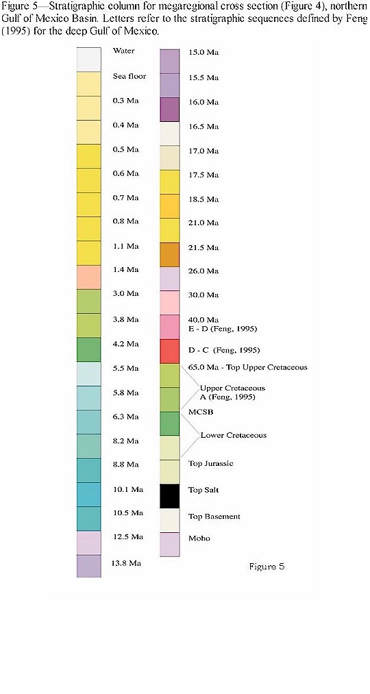
Figure 5—Stratigraphic column for megaregional
cross section (Figure 4), northern Gulf of Mexico Basin.
Letters refer to the stratigraphic sequences defined by Feng (1995) for the deep Gulf of
Mexico.
Figure 6(see animation)—Multiple
structural restorations (using GeoSec) illustrating technique sensitivity to essential
factors that need to be considered during restoration. Present-day geometry is the same in
each column; restorations vary depending on which factors (isostatics, paleobathymetry,
decompaction) are incorporated. Ignoring these factors causes reconstructed salt
thicknesses to be too thick and changes the timing of salt weld formation, two critical
parameters in conducting thermal modeling and petroleum migration analyses. Salt is black;
water is shaded.
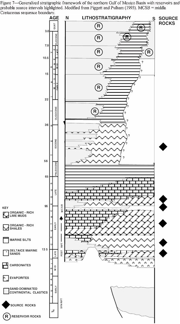
Figure 7—Generalized stratigraphic framework of the
northern Gulf of Mexico Basin with reservoirs and probable source intervals highlighted.
Modified from Piggott and Pulham (1993). MCSB = middle Cretaceous sequence boundary.
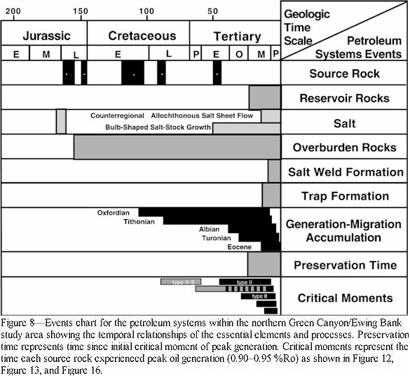
Figure 8—Events chart for the petroleum systems
within the northern Green Canyon/Ewing Bank study area showing the temporal relationships
of the essential elements and processes. Preservation time represents time since initial
critical moment of peak generation. Critical moments represent the time each source rock
experienced peak oil generation (0.90–0.95 %Ro) as shown in Figure 12, Figure 13,
and Figure 16.
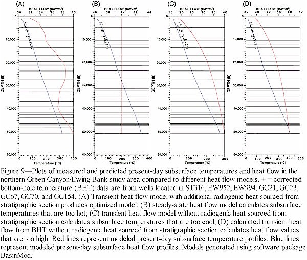
Figure 9—Plots of measured and predicted
present-day subsurface temperatures and heat flow in the northern Green Canyon/Ewing Bank
study area compared to different heat flow models. + = corrected bottom-hole temperature
(BHT) data are from wells located in ST316, EW952, EW994, GC21, GC23, GC67, GC70, and
GC154. (A) Transient heat flow model with additional radiogenic heat sourced from
stratigraphic section produces optimized model; (B) steady-state heat flow model
calculates subsurface temperatures that are too hot; (C) transient heat flow model without
radiogenic heat sourced from stratigraphic section calculates subsurface temperatures that
are too cool; (D) calculated transient heat flow from BHT without radiogenic heat sourced
from stratigraphic section calculates heat flow values that are too high. Red lines
represent modeled present-day subsurface temperature profiles. Blue lines represent
modeled present-day subsurface heat flow profiles. Models generated using software package
BasinMod.
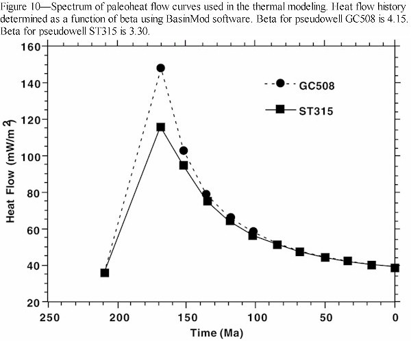
Figure 10—Spectrum of paleoheat flow curves used in
the thermal modeling. Heat flow history determined as a function of beta using BasinMod
software. Beta for pseudowell GC508 is 4.15. Beta for pseudowell ST315 is 3.30.
Figure 11—Transformation ratio calculations (from BasinMod)
of potential source rocks in Green Canyon 112 (A–D) and Ewing Bank 950 (E–I)
pseudo-wells:
Turonian, and (I) EW950 Eocene. Green lines represent tops and
bottoms of standard type II
kerogen source rocks, red lines
represent tops and bottoms of type II-S (Monterey) kerogen source rocks, blue lines
represent tops
and bottoms of type II-S (Kirkuk) kerogen source rocks (Table 3)
(Tissot et al., 1987). Locations are shown in Figure 14.
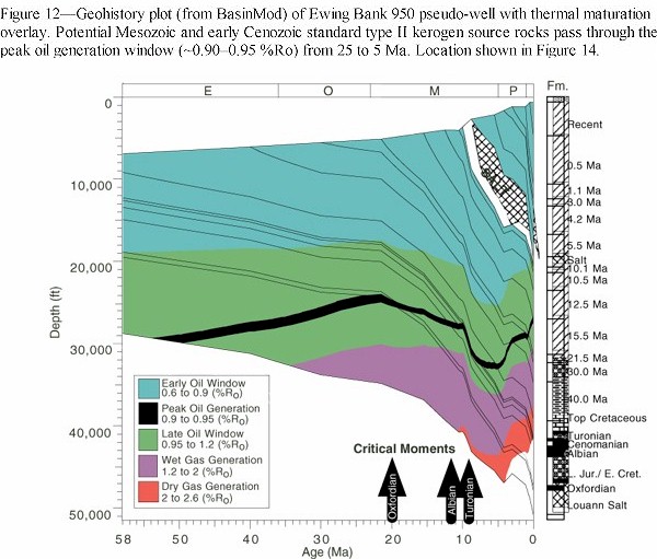
Figure 12—Geohistory plot (from BasinMod) of Ewing
Bank 950 pseudo-well with thermal maturation overlay. Potential Mesozoic and early
Cenozoic standard type II kerogen source rocks pass through the peak oil generation window
(~0.90–0.95 %Ro) from 25 to 5 Ma. Location shown in
Figure 14.
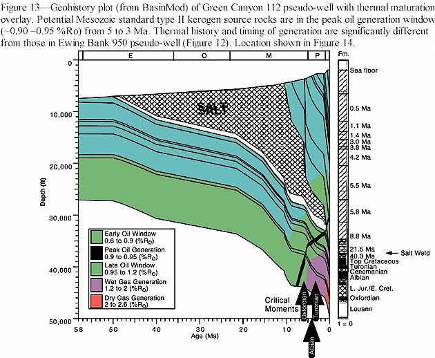
Figure 13—Geohistory plot (from BasinMod) of Green
Canyon 112 pseudo-well with thermal maturation overlay. Potential Mesozoic standard type
II kerogen source rocks are in the peak oil generation window (~0.90 –0.95 %Ro)
from 5 to 3 Ma. Thermal history and timing of generation are significantly different from
those in Ewing Bank 950 pseudo-well (Figure 12).
Location shown in Figure 14.
Figure 14(see animation)—Structural
restorations (identical to Figure 4) with superimposed thermal
maturation windows across northern Green Canyon from 15.5 Ma to the present. Section
location shown on Figure 3; vertical lines indicate locations
of BasinMod one-dimensional thermal models, including those shown in Figure 12 and Figure 13.
Combination of thermal maturation modeling and structural restorations illustrates the
effect of the original salt geometry, evolution, and evacuation on the subsalt thermal
maturation.
Consequently, the critical moment of peak oil generation for each of the potential
Mesozoic and early Cenozoic sources varies spatially and temporally along the line of
section. For example, generation is retarded beneath the central salt stock until weld
formation (15.5–3.0 Ma), and at the southern end of section after sheet emplacement
(5.5–0 Ma). Color legend for thermal maturation windows is the same as in Figure 12 and Figure 13.
Salt is black.
Figure 15(see animation)—1:1
depth section and sequential restorations of seismic profile C from regional study area
(see Figure 3 for location). The restorations show the
evolution of a central salt stock into a bowl-shaped minibasin, and how this evolution
influenced petroleum migration pathways through time. Arrows represent petroleum migration
pathways at the time of each restoration. Migration is believed to be vertical until it
reaches the base of salt (in black), at which point it is deflected up the dip along the
base of salt. Vertical migration is believed to resume when and where salt welds form. The
evolution of salt concentrates petroleum migration in some regions through time, whereas
salt shields suprasalt sediments from petroleum migration for significant amounts of time.
Changes in length of suprasalt section show amounts of extension and contraction.
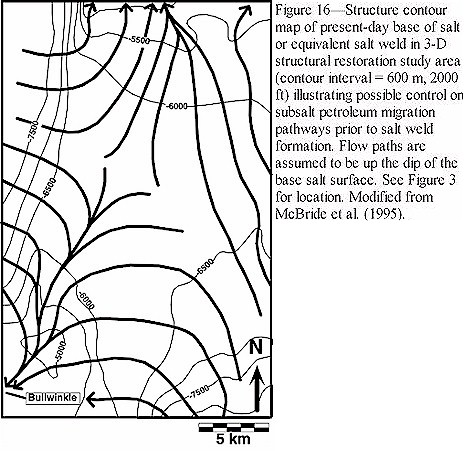
Figure 16—Structure contour map of present-day base
of salt or equivalent salt weld in 3-D structural restoration study area (contour interval
= 600 m, 2000 ft) illustrating possible control on subsalt petroleum migration pathways
prior to salt weld formation. Flow paths are assumed to be up the dip of the base salt
surface. See Figure 3 for location. Modified from McBride et
al. (1995).
Figure 17(see animation of
Figures 3, 17, and 18)—Reconstructed subsalt petroleum migration pathways map.
Arrows show flow paths up the dip of interpreted base salt. Zones of flow concentration
highlighted with flow cells outlined by heavy lines. The map represents diachronous
allochthonous salt distribution and does not represent a discrete moment in time.
Locations of fields and discoveries also are shown to illustrate their correspondence to
original subsalt petroleum migration concentrations. See text for discussion.
Figure 18(see animation of
Figures 3, 17, and 18)—Present-day subsalt petroleum migration pathways map.
Present-day salt distribution is shaded, with arrows showing subsalt flow paths. White
represents salt welds, which are regions of vertical petroleum migration. Locations of
fields and discoveries are shown to illustrate spatial positioning near edges of
allochthonous salt (suprasalt) or where flow is concentrated (subsalt). See text for
discussion.
Tables
Table 1. Fields and Discoveries of the Northern Green Canyon/Ewing
Bank Study Area
Table 2. Input Parameters for Thermal Maturation Modeling Using
BasinMod
Table 3. Kinetic Parameters for Standard Type II and Type II-S
Kerogens*
 Figure 1—Location map of study area, northern Green
Canyon and Ewing Bank, northern Gulf of Mexico.
Figure 1—Location map of study area, northern Green
Canyon and Ewing Bank, northern Gulf of Mexico.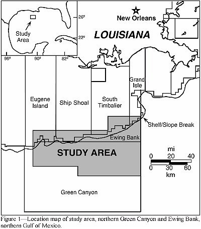