|
Introduction
Figure
Captions (1-2.1 - 1-2.3)
 Figure 1-2.1. Location of study area: western
part of Great Divide basin and Rawlins-Sierra Madre uplift. Figure 1-2.1. Location of study area: western
part of Great Divide basin and Rawlins-Sierra Madre uplift.
 Figure 1-2.2. Paleogeographic map for lower
Maastrictian (approximately 69.4 Ma) (after McGookey et al., 1972). Figure 1-2.2. Paleogeographic map for lower
Maastrictian (approximately 69.4 Ma) (after McGookey et al., 1972).
 Figure 1-2.3. Upper Cretaceous stratigraphy,
south-central Wyoming (after Schell, 1973). Figure 1-2.3. Upper Cretaceous stratigraphy,
south-central Wyoming (after Schell, 1973).
The ultimate goal of this research is to
develop sequence stratigraphic-based models for predicting seal
occurrence and estimating top seal capacity for application in
hydrocarbon exploration and risk analysis. Few systematic studies of
seal character and shale sedimentology are available. Consequently,
seals remain the least understood element of petroleum systems.
The Lewis Shale (Upper Cretaceous,
Maastrichtian), which crops out along the eastern margins of the Great
Divide and Washakie basins in south-central Wyoming, provides an
interesting analog for understanding stratigraphic architecture of
turbidite depositional systems (Figures 1-2.1,
1-2.2, and 1-2.3).
Previous outcrop and subsurface studies (e.g., Pyles and Slatt, 2000)
established a high-frequency sequence stratigraphic framework for the
Lewis Shale. Winton-Barnes et al. (2000) characterized sandstone
lithotypes within the Lewis Shale, and Costeblanco-Torres (2003)
completed a detailed study of shale lithotypes from Lewis Shale outcrops
and cores. Almon et al. (2002) documented considerable variability in
petrophysical properties of shales within the Lewis Shale.
The Lewis Shale is exposed intermittently
along a 60-mile-long outcrop belt on the Rawlins-Sierra Madre uplift
west of Cheyenne, Wyoming (1-2.1). Extensive subsurface data are
provided by numerous producing fields west of the outcrop belt.
Stratigraphy
(Figures 3.1-3.5)
Figure
Captions (3.1-3.5)
 Figure 3.1. Champlin 276 D-1, Section 13,
T19N, R93W, Carbon County, Wyoming. Photograph of the core showing
black, organic, fissile shale with laminated bentonite beds, together
with section of well log containing cored interval (from that part of
the Lewis Shale representative largely of aggradation). Figure 3.1. Champlin 276 D-1, Section 13,
T19N, R93W, Carbon County, Wyoming. Photograph of the core showing
black, organic, fissile shale with laminated bentonite beds, together
with section of well log containing cored interval (from that part of
the Lewis Shale representative largely of aggradation).
 Figure 3.2. Sierra Madre outcrop, Section
24/25, T16N, R92W, Carbon County, Wyoming. Photographs of outcrop area
and log of stratigraphic interval examined (from that part of the Lewis
Shale representative largely of progradation). Figure 3.2. Sierra Madre outcrop, Section
24/25, T16N, R92W, Carbon County, Wyoming. Photographs of outcrop area
and log of stratigraphic interval examined (from that part of the Lewis
Shale representative largely of progradation).
 Figure 3.3. High-frequency sequence
stratigraphic cross section of Lewis Shale, south-central Wyoming, with
location and position of core in Figure 3.1
and of outcrop interval in
Figure 3.2. (Modified after Pyles and Slatt, 2000). Figure 3.3. High-frequency sequence
stratigraphic cross section of Lewis Shale, south-central Wyoming, with
location and position of core in Figure 3.1
and of outcrop interval in
Figure 3.2. (Modified after Pyles and Slatt, 2000).
 Figure 3.4. Upper Cretaceous stratigraphic
framework in terms of time, sequence stratigraphy, and polarity. Figure 3.4. Upper Cretaceous stratigraphic
framework in terms of time, sequence stratigraphy, and polarity.
 Figure 3.5. Relation between eustatic cycles,
depositional geometry cycles, and systems tracts (modified after Rahmanian et al., 1990). Figure 3.5. Relation between eustatic cycles,
depositional geometry cycles, and systems tracts (modified after Rahmanian et al., 1990).
Return
to top.
High-frequency sequence stratigraphic cross-section reveals that the
Lewis Shale consists of at least twenty (probable 4th-order)
depositional sequences (Figure 3.3). Beneath the “Asquith Marker” Lewis
Shale deposition was basically aggradational (Figure 3.1). The overlying progradational unit consists dominantly of silty shales (3rd-order
highstand [HST]) with interstratified 4th-order “lowstand” (LST)
sandstones (Figure 3.2). These sandstones record below storm wave base
deposition from storm-induced gravity flows. Relatively weak seals (HST
shales) are interstratified with the sandstones (potential reservoirs).
Champlin 276 D-1, Section 13, T19N, R93W,
Carbon County, Wyoming
Figure Captions
(4.1-4.2)
 Figure 4.1. Mercury injection capillary
pressure curves, pore size distribution, photomicrographs, and SEM
photographs for representative core samples, from the TST part of the
Lewis Shale, in Champlin 276 D-1, together with section of well log that
shows calibrated cored interval and positions of samples.
Samples are
from microfacies 1 (finely laminated, pyritic, black shales) and
microfacies 4 (fossiliferous, slightly to moderately silty claystones). Figure 4.1. Mercury injection capillary
pressure curves, pore size distribution, photomicrographs, and SEM
photographs for representative core samples, from the TST part of the
Lewis Shale, in Champlin 276 D-1, together with section of well log that
shows calibrated cored interval and positions of samples.
Samples are
from microfacies 1 (finely laminated, pyritic, black shales) and
microfacies 4 (fossiliferous, slightly to moderately silty claystones).
 Figure
4.2. (Left) Major constituents of Lewis Shale in cored interval in
Champlin 276 D-1. (Right) Clay-mineral composition of Lewis Shale in
cored interval in Champlin 276 D-1. Figure
4.2. (Left) Major constituents of Lewis Shale in cored interval in
Champlin 276 D-1. (Right) Clay-mineral composition of Lewis Shale in
cored interval in Champlin 276 D-1.
The Champlin 276 D-1 core (Figure 4.1)
represents the transgressive (TST) part of the Lewis Shale. These
samples have significantly higher MICP values (mean 18,000 psia)
relative to other Lewis Shale samples (Figure 4.1). Shales exhibiting
well-developed laminar fabrics and enrichment in iron-bearing clay
minerals, TOC, and authigenic pyrite have excellent to exceptional
seal.
Total clay content varies from 54 to 64
percent (Figure 4.2) with a mean of 51 percent (std dev = 2.5 %). Quartz
content ranges from 23 to 34 percent. The mean is 28 percent (std dev =
3.9 %). Detrital feldspars, pyrite, and carbonate are common accessory
(18 to 26 percent; mean 20) minerals. The dominant clay type is the 2:1
aluminum family (Figure 4.2). Abundance ranges from 17 to 32 percent
with a mean of 25 (std dev = 5.1 %). The 2:1 iron-bearing clays are also
major components. Their abundance ranges from 15 to 27 percent with a
mean of 21 percent (std dev = 4.6 %). Kaolinite (mean 4 %) and
iron-bearing chlorite (mean = 1%) are minor components.
Sierra Madre Outcrop
Section 25/25, T16N, R92W, Carbon County,
Wyoming
Figure Captions
(5.1-5.3)
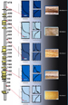 Figure 5.1. Mercury injection capillary
pressure curves, pore size distribution, and photomicrographs for
representative samples from the HST part of the Lewis Shale,
Sierra
Madre outcrop, together with log of stratigraphic interval and positions
of samples. Samples are from microfacies 2 (moderately to very silty
calcareous shales) and microfacies 5 (very silty shales and mottled
argillaceous siltstones). Figure 5.1. Mercury injection capillary
pressure curves, pore size distribution, and photomicrographs for
representative samples from the HST part of the Lewis Shale,
Sierra
Madre outcrop, together with log of stratigraphic interval and positions
of samples. Samples are from microfacies 2 (moderately to very silty
calcareous shales) and microfacies 5 (very silty shales and mottled
argillaceous siltstones).
 Figure
5.2. Photographs of outcrop area. A. General view. B. HST shale (15 cm
scale). C. Sandstone-filled channel within HST shale. D. Sheet sandstone
within HST shale. Figure
5.2. Photographs of outcrop area. A. General view. B. HST shale (15 cm
scale). C. Sandstone-filled channel within HST shale. D. Sheet sandstone
within HST shale.
 Figure 5.3. (Left) Major consitituents of
Lewis Shale in Sierra Madre outcrop. (Right) Clay-mineral composition of
Lewis Shale in Sierra Madre outcrop. Figure 5.3. (Left) Major consitituents of
Lewis Shale in Sierra Madre outcrop. (Right) Clay-mineral composition of
Lewis Shale in Sierra Madre outcrop.
The Sierra Madre outcrop represents the highly
progradational (3rd-order highstand) part of the Lewis Shale; the
dominant lithofacies are silty shales (microfacies 2) and argillaceous
siltstones (microfacies 5) (Figure
5.1). Several high-frequency (4th- or
5th-order) lowstand sandstone units are interstratified with this
highstand systems tract (HST). Two major types of sandstone bodies (lenticular
and tabular) are recognizable in this outcrop (Witton-Barnes, 2000)
(Figure 5.2).
Massive
to weakly laminated shales and siltstones that compose the Lewis Shale
HST are characterized by relatively high (mean 37 %) content of detrital
silt, low TOC values, and the lowest sealing capacities (mean 1.150 psia)
measured within the Lewis Shale (Figure
5.1). These relatively low
sealing capacities are typical of shales from proximal parts of marine
depositional systems (Dawson and Almon, 2002).
Total clay content ranges from 35 to
71% (mean 52%) (Figure
5.3). Detrital silt (quartz + feldspars)
abundance varies from 24 to 59% (mean 37%). Pyrite, siderite,
Mg-calcite, and dolomite are accessory (1 to 4%) components. The
normalized clay mineral composition is dominated (56 to 78%) by 2:1
aluminum clays (mean 67%) (Figure
5.3).
Return
to top.
Colorado School of Mines
Stratigraphic Test 61
Section 25, T16N, R92W,
Carbon County, Wyoming
Figure Captions (6.1-6.2)
 Figure 6.1. Mercury injection capillary
pressure curves, pore size distribution, photographs, photomicrographs,
and SEM photographs for representative core samples,
from the LST part
of the Lewis Shale, in Colorado School of Mines Strat Test 61, together
with wireline log that shows positions of samples.
Samples are from microfacies 2 (moderately to very silty calcareous shales), microfacies
3 (moderately to very silty, mottled, calcareous shales), microfacies 4
(fossiliferous, slightly to moderately silty claystones), and
microfacies 5 (very silty shales and mottled argillaceous siltstones). Figure 6.1. Mercury injection capillary
pressure curves, pore size distribution, photographs, photomicrographs,
and SEM photographs for representative core samples,
from the LST part
of the Lewis Shale, in Colorado School of Mines Strat Test 61, together
with wireline log that shows positions of samples.
Samples are from microfacies 2 (moderately to very silty calcareous shales), microfacies
3 (moderately to very silty, mottled, calcareous shales), microfacies 4
(fossiliferous, slightly to moderately silty claystones), and
microfacies 5 (very silty shales and mottled argillaceous siltstones).
 Figure 6.2. (Left) Major constituents of Lewis
Shale in Colorado School of Mines Strat Test 61. (Right) Clay-mineral
composition of Lewis Shale in Colorado School of Mines Strat Test 61. Figure 6.2. (Left) Major constituents of Lewis
Shale in Colorado School of Mines Strat Test 61. (Right) Clay-mineral
composition of Lewis Shale in Colorado School of Mines Strat Test 61.
Samples from the Colorado School of Mines
Strat Test 61 represent the lowstand Lewis Shale. These samples consist
of very silty shales and siltstones that have relatively low MICP values
(mean 2886 paia). Lower MICP values are typical of silt-rich shales
wherein detrital sized grains are concentrated into high-frequency
laminae (Figure
6.1).
Total
clay content varies from 35 to 69 percent (Figure
6.2) with a mean of 51
percent (std dev = 8.5 %). Quartz content ranges from 3 to 41 percent.
The mean is 27 percent (std dev = 8.6 %). Detrital feldspars, pyrite and
carbonate are common accessory (16 to 32 percent; mean 21) minerals. The
dominant clay type is the 2:1 aluminum family. Abundance ranges from 0
to 46 percent with a mean of 31 (std dev = 5.1 %). The 2:1 iron-bearing
clays are also major components (Figure
6.2). Their abundance ranges
from 7 to 24 percent with a mean of 14 percent (std dev = 3.8 %). Kaolinite (mean 6 %) and iron-bearing chlorite (mean = 1%) are minor
components.
Figure Captions (7.1-7.8)
 Figure 7.1. Microfacies of the Lewis Shale and
some of their characteristics. Figure 7.1. Microfacies of the Lewis Shale and
some of their characteristics.
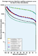 Figure 7.2. Average mercury injection
capillary pressure curve for each of the five microfacies of the Lewis
Shale, with TST showing the best seal character. Figure 7.2. Average mercury injection
capillary pressure curve for each of the five microfacies of the Lewis
Shale, with TST showing the best seal character.
 Figure
7.3. Canonical discriminant analysis distinguishes the five Lewis Shale
microfacies, which are illustrated by photomicrographs. Figure
7.3. Canonical discriminant analysis distinguishes the five Lewis Shale
microfacies, which are illustrated by photomicrographs.
 Figure 7.4. Iron 2:1 clay content of TST and
HST shales plotted against MICP @ 10% saturation (psia), with the former
showing higher values. Figure 7.4. Iron 2:1 clay content of TST and
HST shales plotted against MICP @ 10% saturation (psia), with the former
showing higher values.
 Figure 7.5. Plot of porosity of TST and HST
shales, with the former showing lower values. (MFS=maximum flooding
surface.) Figure 7.5. Plot of porosity of TST and HST
shales, with the former showing lower values. (MFS=maximum flooding
surface.)
 Figure 7.6. Plot of 10%MICP saturation of
Lewis Shale samples according to depositional systems, with TST shales,
condensed shales, and paleosols showing the greatest seal capacity. Figure 7.6. Plot of 10%MICP saturation of
Lewis Shale samples according to depositional systems, with TST shales,
condensed shales, and paleosols showing the greatest seal capacity.
 Figure 7.7. Plot of porosity and permeability
shows a strong correlation between subsurface and surface samples. Figure 7.7. Plot of porosity and permeability
shows a strong correlation between subsurface and surface samples.
 Figure 7.8. Tmax values of TST and HST shales
are effectively the same. Figure 7.8. Tmax values of TST and HST shales
are effectively the same.
Return
to top.
Five microfacies have been recognized in the
Lewis Shale in the study area; they are tabulated in
Figure 7.1 and
listed below:
-
Microfacies 1--Finely
laminated, pyritic, black shales. Excellent seal character.
Depositional system: TST/CI.
-
Microfacies 2--Moderately
to very silty calcareous shales. Poor seal character. Depositional
system: HST.
-
Microfacies 3--Moderately
to very silty, mottled, calcareous shales Moderate to poor seal
character. Depositional system: LST.
-
Microfacies
4--Fossiliferous slightly to moderately silty claystones Variable seal
character. Depositional system: TST/HST.
-
Microfacies 5--Very silty
shales and mottled argillaceous siltstones. Poor seal character.
Depositional system: HST/LST.
Distal marine (TST) shales (microfacies 1 and 4) exhibit the “best” seal
character based on MICP analysis (Figure 7.2). Discriminant function
analysis of Lewis Shale microfacies yielded two functions that account
for nearly 99% of the total variance (Figure 7.3).
TST shales are enriched in
iron-bearing clay minerals and pyrite and have strongly elevated MICP
values relative to HST shales (Figure 7.4).
Porosity
of TST shales is significantly lower than porosity in HST shales (Figure
7.5). MICP values are increased as porosity is reduced significantly in
the upper TST interval relative to all parts of the HST interval. The
reduced porosity in clay-rich TST shales is attributed to improved
organization of particles (well-developed laminar fabrics) as well as
the precipitation of Fe-carbonate cements during early submarine
diagenesis.
Additionally, there is a major difference in the permeability of TST and
HST shales. Within the Lewis HST there is a weak trend of upward
increasing permeability; this trend appears to correlate with a vertical
increase in the content of detrital silt. There is a correlation between
seal capacity and depositional systems, with an progressive increase in
capacity from slumps/debris flows, HST, MFS, TST, condensed shales, to
paleosols (Figure 7.6).
A strong correlation between subsurface and
outcrop samples, along with evidence of comparable burial history (Tmax
data), suggests that other factors (e.g., diagenetic processes) are
responsible for differences in seal character (Figure 7.7). Tmax values
are essentially the same for all Lewis Shale samples; this implies that
they have undergone comparable burial histories (Figure 7.8).
Figure Captions (8.1-8.10)
 Figure 8.1. Bulk density of TST shales greatly
exceeds the bulk density of HST shales. Figure 8.1. Bulk density of TST shales greatly
exceeds the bulk density of HST shales.
 Figure 8.2. Poisson’s ratio in TST shales is
generally less than Poisson’s ratio of HST shales. Figure 8.2. Poisson’s ratio in TST shales is
generally less than Poisson’s ratio of HST shales.
 Figure 8.3. Shear velocity of TST shales
exceeds the maximum shear velocity of HST shales. Figure 8.3. Shear velocity of TST shales
exceeds the maximum shear velocity of HST shales.
 Figure 8.4. HST shales exhibit an overall
increase in compressional velocity above the MFS. The average
compressional velocity of TST shales is approximately equal to the
maximum HST compressional velocity. Figure 8.4. HST shales exhibit an overall
increase in compressional velocity above the MFS. The average
compressional velocity of TST shales is approximately equal to the
maximum HST compressional velocity.
 Figure 8.5. Data used for seismic model. Figure 8.5. Data used for seismic model.
 Figure 8.6. Synthetic seismogram for model 1. Figure 8.6. Synthetic seismogram for model 1.
 Figure 8.7. Synthetic seismogram for model 2. Figure 8.7. Synthetic seismogram for model 2.
 Figure 8.8. Synthetic seismogram for model 3. Figure 8.8. Synthetic seismogram for model 3.
 Figure 8.9. Comparison of the seismic data
from model 1 (red) and model 3 (green) shows the relatively minor effect
of removing the orange and green layers. Figure 8.9. Comparison of the seismic data
from model 1 (red) and model 3 (green) shows the relatively minor effect
of removing the orange and green layers.
 Figure 8.10. Seismic profile, with features of
high-reflectivity shale resembling those of sandstone saturated with
hydrocarbons. Figure 8.10. Seismic profile, with features of
high-reflectivity shale resembling those of sandstone saturated with
hydrocarbons.
Return
to top.
Rock Properties
Measurements reveal significant differences in the bulk density,
Poisson’s ratio, and shear velocity of TST and HST shales (Figures
8.1,
8.2, and 8.3). The differences in rock properties across a shale-shale
contact (i.e., low velocity and low density HST shale immediately above
a high velocity and high density TST shale—Figures
8.1, 8.3, and
8.4)
could generate a strong seismic reflection.
Shale Reflection Modeling Experiment
The basic modeling performed in this
experiment used measured elastic rock properties data and layer
thicknesses from well logs (Figure 8.5). Angle-specific reflection
coefficients were computed for all interfaces and for angles ranging
from 0 to 60 degrees. The result was an angle gather of reflection
coefficients.
Each trace of this gather represents a
specific reflection angle and was convolved with an angle-specific
wavelet. These wavelets were derived from analog well data and
stretched/squeezed to simulate the effect of NMO. The result is a
synthetic seismic angle gather that shows the AVA effect of the gather
(model 1--Figure 8.6).
To assess the effect of the thin
high-impedance shale (orange layer), it was removed, and the
calculations repeated without it. The result (model 2--Figure 8.7) shows
that the overall effect on the synthetic seismic is minimal. After
removing both the orange and green layers (model 3--Figure 8.8), the
effect is more noticeable but remains small (Figure 8.9).
The example of a seismic profile in
Figure
8.10 shows a shale horizon (strong seismic reflector) that could be
misinterpreted as hydrocarbon-saturated sandstone. Results from a well
confirm the absence of sandstone.
Figure Caption (9.1)
 Figure 9.1. Wireline log of LST reservoir,
immediately overlain by waste-zone shale composed microfacies 2 and
microfacies 3, which in turn is overlain by the top-seal shale, composed
of microfacies 4. Figure 9.1. Wireline log of LST reservoir,
immediately overlain by waste-zone shale composed microfacies 2 and
microfacies 3, which in turn is overlain by the top-seal shale, composed
of microfacies 4.
Lewis Shale strata consist of at least 5
argillaceous microfacies that exhibit distinctive sedimentological and
petrophysical features along with significant variations in seal
character.
Uppermost transgressive and condensed shales
(Lewis Shale microfacies 1 and 4) offer excellent to exceptional top
seal potential. These shales occur preferentially in distal parts of
marine depositional systems.
The top seal capacity of highstand (Lewis
Shale microfacies 2 and 5) and lowstand (Lewis Shale microfacies 3 and
5) intervals is reduced mainly because of elevated content (> 25%) of
detrital silt and disrupted fabrics (extensive bioturbation).
Significant stratigraphic separation (several
hundred feet) can exist between a lowstand sandstone reservoir and its
controlling top seal horizon (i.e., overlying transgressive shale)
(Figure 9.1).
Factors that tend to enhance sealing
characteristics of marine shales include: low content (<25%) of detrital silt; relatively slow rates of accumulation; low oxygen levels
and limited bioturbation (preservation of laminar fabrics); and
increasing content of Fe- and Mg-enriched minerals.
Seismically significant parameters (e.g.,
density, shear velocity, Poisson’s ratio, and compressional velocity)
exhibit systematic variations that are consistent within the 3rd-order
sequence stratigraphic framework of the Lewis Shale.
Seismic modeling reveals a potential of some
shales to exhibit an AVO response comparable to that exhibited by
hydrocarbon-saturated sandstones.
Almon, W.R., and Thomas, J.B., 1991, Pore
systems aspects of hydrocarbon trapping: in Gluskloter, H. J., et
al., (eds), Economic Geology of North America, v. P-2, Geological
Society of America, Boulder, CO., p. 241-254.
Almon, W.R., et al., 2002, Sequence
stratigraphy, facies variation and petrophysical properties in deepwater
shales, Upper Cretaceous Lewis Shale, south-central Wyoming: GCAGS
Transactions, v. 52, p. 1041-1053.
Castelblanco-Torres, B., 2003, Distribution of
sealing capacity within a sequence stratigraphic framework: Upper
Cretaceous Lewis Shale, south-central Wyoming: M.S. Thesis, Colorado
State University.
Dawson, Wm. C., 2000, Shale microfacies: Eagle
Ford Group (Cenomanian-Turonian) north-central Texas outcrops and
subsurface equivalents: GCAGS Transactions, v. 50, p. 607-621.
Dawson, Wm. C., and Almon, W.R., 2002, Top
seal potential of Tertiary deepwater Gulf of Mexico shales: GCAGS
Transactions, v. 52, p. 1657-176.
Dewhurst, D. N., et al., 1999, Permeability
and flow in natural mudstones: in Aplin, A.C., et al. (eds), Muds
and mudstones-Physical Properties: Special Publication 38, Geological
Society of London, p. 23-43.
Jennings, J.J., 1987, Capillary pressure
techniques; application to exploration and development geology: AAPG
Bulletin, v. 71, p. 1196-1209.
Katsube, T.J., and Williamson, M.A., 1994,
Effects of diagenesis on shale nano-pore structure and implications for
sealing capacity: Clay Minerals, v. 29, p. 451-461.
Pyles, D.R., and Slatt, R.M., 2000, A
high-frequency sequence stratigraphic framework for the Lewis Shale and
Fox Hill Sandstone, Great Divide and Washakie basins: GCSEPM Foundation
20th Annual Research Conference, p. 836-861.
Rahmanian, V.D., More, P.S., Mudge, W.J., and
Spring, D.E., 1990, Sequence stratigraphy and the habitat of
hydrocarbons, Gippsland Basin, Australia, in Brooks, J., (ed),
Classic Petroleum Provinces: Geological Society of London Special
Publication no. 50, p. 525-544.
Schieber, J., 1999, Distribution of mudstone
facies in the Upper Devonian Sonyea Group of New York: Journal
Sedimentary Petrology, v. 69, p. 909-925.
Showalter, T. T., 1979, Mechanics of secondary
hydrocarbon migration: AAPG Bulletin, v. 63, p. 723-760.
Winn, R. D., et al., 1987, Shallow-water and
sub-storm-base deposition of Lewis Shale in Cretaceous Western Interior
Seaway, south-central Wyoming: AAPG Bulletin, v. 71, p. 859-881.
Winton-Barnes, E. M., et al., 2000, Outcrop
and subsurface criteria for the differentiation of sheet and
channel-fill strata: example from the Cretaceous Lewis Shale, Wyoming:
GCSEPM Foundation 20th Annual Research Conference, p. 1087-1104.
The authors thank ChevronTexaco for permission
to present these data and interpretations. We are especially grateful to
R.M. Slatt, D.R. Pyles and S.M. Goolsby for sharing their knowledge
concerning the Lewis Shale. C.W. Ward aided with the collection of
samples. W.T. Lawrence prepared thin sections, and J.L. Jones
contributed SEM images. D.K. McCarty completed XRD analyses, and Poro-Technology
(Houston, TX) provided MICP analyses. Graphic design by L.K. Lovell (ChevronTexaco).
Return
to top.
|