|
Figure
Captions
 Figure 1.
The VSP tool shown above consists of 12
individual sondes linked by an electronic cable and terminated with a
logging cable head.
The distance between each sonde can be 10, 15 or 20 m.
Each sonde contains three orthogonal geophones (two horizontal and one
vertical) and a single hydrophone.
A hydraulically powered locking arm
(shown retracted) ensures that the geophone package is secured against the
borehole wall. (Photograph furnished by CGG.) Figure 1.
The VSP tool shown above consists of 12
individual sondes linked by an electronic cable and terminated with a
logging cable head.
The distance between each sonde can be 10, 15 or 20 m.
Each sonde contains three orthogonal geophones (two horizontal and one
vertical) and a single hydrophone.
A hydraulically powered locking arm
(shown retracted) ensures that the geophone package is secured against the
borehole wall. (Photograph furnished by CGG.)
 Figure 2.
Example geometries of surface source and sondes
(containing the geophone package).
A
survey should be planned with the travelpath of the seismic energy in mind.
A far-offset VSP field setup
such as a source at S2 and receiver at A would image the
interface at the borehole if the position A was at the interface and up to
half the offset distance along the interface if the geophone position A
was at the surface. Figure 2.
Example geometries of surface source and sondes
(containing the geophone package).
A
survey should be planned with the travelpath of the seismic energy in mind.
A far-offset VSP field setup
such as a source at S2 and receiver at A would image the
interface at the borehole if the position A was at the interface and up to
half the offset distance along the interface if the geophone position A
was at the surface.
 Figure 3.
The full wavefield (both up- and downgoing Figure 3.
The full wavefield (both up- and downgoing  events events ) zero-offset VSP data in
(A) shows high amplitude downgoing events.
The upgoing events in (B) can
only be seen easily after wavefield separation (downgoing waves are
isolated and subtracted out of the data).
In (C), the upgoing events are
aligned in two-way traveltime (+TT) and can be tied to the surface seismic
stacked section.
The upgoing event colored orange intersects the first
break curve at the trace representing the depth of the interface which
caused the reflection. ) zero-offset VSP data in
(A) shows high amplitude downgoing events.
The upgoing events in (B) can
only be seen easily after wavefield separation (downgoing waves are
isolated and subtracted out of the data).
In (C), the upgoing events are
aligned in two-way traveltime (+TT) and can be tied to the surface seismic
stacked section.
The upgoing event colored orange intersects the first
break curve at the trace representing the depth of the interface which
caused the reflection.
 Figure 4.
On a zero- or near-offset VSP, the upgoing
reflected event travels down to the reflecting interface and up to the
sonde containing the geophones. If the raypath had continued to the
surface along the additional blue line, the event would be in two-way
traveltime.
The traveltime along the blue path is the first break time for
zero-offset geometry. By adding this time to the trace recorded at the sonde, the VSP data is placed into pseudo two-way traveltime. Figure 4.
On a zero- or near-offset VSP, the upgoing
reflected event travels down to the reflecting interface and up to the
sonde containing the geophones. If the raypath had continued to the
surface along the additional blue line, the event would be in two-way
traveltime.
The traveltime along the blue path is the first break time for
zero-offset geometry. By adding this time to the trace recorded at the sonde, the VSP data is placed into pseudo two-way traveltime.
 Figure 5.
The deconvolved upgoing events in (B) show that the VSP deconvolution has
been fairly successful when applied to the data in (A). The purple event
at about 1.16 s is now continuous across all traces. Some residual
multiple contamination remains on the shallow depth traces. Figure 5.
The deconvolved upgoing events in (B) show that the VSP deconvolution has
been fairly successful when applied to the data in (A). The purple event
at about 1.16 s is now continuous across all traces. Some residual
multiple contamination remains on the shallow depth traces.
 Figure 6.
The first break event is found on both the X and
Y data. The wavelet is sometimes more consistent on one compared to the
other. This is due to the tool rotating in the borehole between tool
relocations. The first break event in (A) is the primary downgoing P- or
compressional wave. A mode-converted SV or shear event is highlighted in
blue in panels (A) and (C). This event dips in a different direction than
the downgoing P event because of its slower velocity. In panel (C), the
P-wave up- and downgoing events are easily recognized. Note that near the
bottom of the data panel there is a hyperbolic-shaped event which could be
a refracted shear at the 750 m interface. Figure 6.
The first break event is found on both the X and
Y data. The wavelet is sometimes more consistent on one compared to the
other. This is due to the tool rotating in the borehole between tool
relocations. The first break event in (A) is the primary downgoing P- or
compressional wave. A mode-converted SV or shear event is highlighted in
blue in panels (A) and (C). This event dips in a different direction than
the downgoing P event because of its slower velocity. In panel (C), the
P-wave up- and downgoing events are easily recognized. Note that near the
bottom of the data panel there is a hyperbolic-shaped event which could be
a refracted shear at the 750 m interface.
 Figure 7.
The data in (A) resulted from applying several
data polarization steps to the X, Y, and Z data shown in
Figure 6.
The
isolated upgoing event data is plotted in depth of sonde location (trace)
versus two-way traveltime. In order to visualize the geology extending
from the well laterally towards the source direction, the VSPCDP
transformed data is computed and shown in (B). The data show two faults,
and the green event truncates against the first fault located
approximately 75 meters from the well location. Figure 7.
The data in (A) resulted from applying several
data polarization steps to the X, Y, and Z data shown in
Figure 6.
The
isolated upgoing event data is plotted in depth of sonde location (trace)
versus two-way traveltime. In order to visualize the geology extending
from the well laterally towards the source direction, the VSPCDP
transformed data is computed and shown in (B). The data show two faults,
and the green event truncates against the first fault located
approximately 75 meters from the well location.
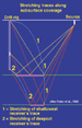 Figure 8.
The VSPCDP transform converts the depth/traveltime
data in
Figure 7(A)
to the lateral offset
away from the well/traveltime data in
Figure 7(B).
This enables one to
interpret subsurface geology between the well and the source. Figure 8.
The VSPCDP transform converts the depth/traveltime
data in
Figure 7(A)
to the lateral offset
away from the well/traveltime data in
Figure 7(B).
This enables one to
interpret subsurface geology between the well and the source.
The
operation of the VSP survey is as follows:
·
The sonde containing the geophone
package of three orthogonal X, Y, and Z geophones (Figure
1) is lowered to a prescribed depth location.
·
A locking arm on the sonde pushes
the geophone assembly against the borehole wall.
·
The surface source energy source
is fired.
Acoustic energy from the source is recorded at the geophone sonde. The
locking arm is then retracted and the sonde is moved to the next depth
location.
Figure 2 illustrates VSP source and
receiver geometries. The near- or zero-offset VSP geometry occurs when the
source lies vertically above the geophones (source S1 and
receiver A in
Figure 2A). A far-offset VSP occurs when
there is substantial offset distance between the vertical projection of
the sonde to the surface and the source (source S2 and geophone
A in
Figure 2A). In deviated boreholes, source
S3 in
Figure 2B can be zero-offset for location
A, but far-offset for location B. In general,
the zero-offset VSPs will seismically image the geology at the borehole,
and the far-offset VSPs will image laterally from the borehole in the
direction toward the surface source.
Return
to top.
In
Figure 2, the raypaths of the acoustic
energy shown are reflections up from interfaces located below the sonde.
Surface seismic surveys also record energy arriving from below the
geophones. Unlike surface seismic surveys, VSP data also contain acoustic
energy traveling downward toward the geophones in the sonde.
"Upgoing" VSP events are
defined as VSP events that decrease in traveltime as the sonde is lowered
down the borehole -- and cease to exist once the sonde is below the
interface from where the reflection took place.
“Downgoing" events are defined as events whose traveltime increases as the
recording depth increases.
An example of zero-offset VSP
data is shown in
Figure 3A. Note that the downgoing events
are much higher amplitude than the upgoing events, which dip in the
opposite direction. The first arriving event (first break curve) is the
primary P-wave downgoing event. A downgoing event arriving later in time
than the primary must be a multiple. The VSP downgoing wavefield contains
all of the multiple events that contaminate our surface seismic data.
Since the downgoing and upgoing events are linked at the interfaces, we
can use the downgoing events to eliminate multiples from our upgoing VSP
data.
The difference in traveltime
between zero-offset VSP upgoing events (shown in
Figure 3B) and the two-way traveltime of
a surface seismic event is the traveltime along a raypath connecting the
sonde location to a surface geophone. This is equivalent to the traveltime
of the primary downgoing event (Figure
4). Bulk shifting each zero-offset VSP trace by its first break
time aligns the upgoing events into pseudo two-way traveltime (Figure
3C).
One
can determine the depth of the geological interface that created the
upgoing event by:
·
Interpreting the upgoing event on
the shallow depth traces out to the trace where the event intercepts the
first break (time of first recorded data).
·
Following the trace up to the top
of the plot to read off its depth value.
(Look at
Figure 3 and do this for the orange
colored upgoing event in panel C. This is the interpretive link between
the geophysical seismic event and its associated geological interface.)
Multiple identification can be
easily done using VSP data. An upgoing multiple is an upgoing VSP event
whose raypath undergoes more than one reflection bounce during its travel
to the sonde. Find the primary upgoing event in
Figure 3C (colored blue) that terminates
at the first break time of the 750-meter depth trace. A multiple upgoing
event whose last upgoing reflection occurred at the 750-meter interface
arrives later in time but also terminates at the 750-meter trace.
Why?
-- When the sonde is lowered below 750 meters, rays traveling upwards from
the 750-meter interface never reach the sonde. The multiples of our
upgoing primary event (blue) in
Figure 3C are
highlighted in yellow. This allows one to interpret multiples, which may
be contaminating later arriving primary upgoing events. Can you see one?
The green-colored upgoing primary generated at 1,180 meters can be seen to
extend from the first break curve to the multiple contaminated data
highlighted in yellow and change in character.
Multiple
elimination can be achieved by using the downgoing events. In
Figure 3A, the multiple downgoing events
parallel the first break curve. We design an operator that will collapse
all of the downgoing events arriving after the primary downgoing event
(first break curve). This operator can be applied to the data in
Figure 3C. The deconvolved upgoing events
can be seen in
Figure 5B. The deconvolved data can be
compared to the surface seismic data to evaluate the residual multiple
contamination left in the processed surface seismic data.
When the surface source is not located
vertically above the downhole receivers, the up- and downgoing traveling
seismic energy arrive at the sonde at angles other than vertical. At any
given sonde location, the up- and downgoing events are distributed onto
all three geophones (two horizontal, X and Y and vertical Z).
In the processing of the
far-offset data, our aim is to separate the downgoing events from the data
and then isolate the upgoing events on a single data panel for
interpretation. In
Figure 2, the far-offset raypaths show
that interfaces will be imaged from the borehole out to half the source
receiver offset. The final upgoing event panel will be processed to take
on the appearance of a seismic line. Look at the X, Y and Z data in
Figure 6. The primary downgoing event is
distributed onto all three panels. As the sonde is lowered to different
depth levels during the VSP survey, the sonde rotates. This rotation
effect can be seen in the inconsistent first break wavelets on the X and Y
panels.
We want to
isolate the upgoing events. To do this, we process the X, Y, and Z data
using polarization filters (mathematically redistributing the up- and
downgoing events into the plane defined by the wellbore and source).
Wavefield separation is performed to isolate the upgoing events. A final
round of polarization processing is performed to isolate the upgoing
events onto a single data panel. Using the X, Y, and Z data contained in
Figure 6 as input, the final isolated
upgoing events are presented in
Figure 7A.
In
Figure 2A, we saw that the far-offset VSP
geometry resulted in reflections along the interface laterally away from
the borehole. In fact, the coverage extends from right at the intersection
of the interface with the borehole (sonde at depth of interface) out to
half the source/well offset (sonde at borehole surface). As the data is
recorded at various downhole locations starting from the surface down to
the depth of the interface, the geology along the interface is
continuously imaged.
To
transform the data in
Figure 7A into a pseudo-seismic section,
we use a model of the velocity around the borehole. With this model, we
stretch or transform every depth trace into the offset from the well/traveltime domain. This procedure, called the VSPCDP mapping, is shown in
Figure 8 for the deepest and shallowest
depth traces. We apply this process to all the traces and then re-bin the
data to look like seismic traces.
domain. This procedure, called the VSPCDP mapping, is shown in
Figure 8 for the deepest and shallowest
depth traces. We apply this process to all the traces and then re-bin the
data to look like seismic traces.
The output of
this process is shown in
Figure 7B. The horizontal axis is now
distance from the well in meters. In
Figure 7B, two faults can be interpreted.
The distance from the well location where the faulting occurs can be
determined using the horizontal axis. The fault nearest the well can be
interpreted to be 75-80 meters away, and the farthest fault is 205 meters
from the well. A seismic event -- highlighted in
green -- can be seen to truncate against the fault nearest the borehole.
The borehole itself is located along the right edge of the plot in
Figure 7B.
The
zero-offset VSP gives us a link between surface seismic and reflector
depths at the borehole location. Interpretation is easy and the geological
logs can be tied confidently to the VSP and then directly to the surface
seismic. The VSP data illuminate multiples clearly.
If one has
access to VSP data in an area where he/she wants to drill an exploration
well, a quick check for the existence of multiples on the VSP data should
be done. This could prevent drilling a dry hole if the interpretation was
based on surface seismic multiples. The far-offset VSP gives information
of the subsurface away from the well. The lateral imaging can be used to
locate missed targets such carbonate reef edges or missed sand channels.
Return
to top.
|