![]() Click to view images in PDF format.
Click to view images in PDF format.
GCSeismic Modeling and Imaging - Making Waves*
By
Phillip Bording1 and Larry Lines2
Search and Discovery Article #40066 (2002)
*Adapted for online presentation from the Geophysical Corner column in AAPG Explorer December, 2000, entitled “Seismic Modeling Makes Waves,” and prepared by the authors. Appreciation is expressed to the author, to R. Randy Ray, Chairman of the AAPG Geophysical Integration Committee, and to Larry Nation, AAPG Communications Director, for their support of this online version.
1Consultant, Hazel Green, Alberta, Canada
2University of Calgary, Alberta ([email protected])
Exploration seismology essentially involves dealing with seismic ![]() wave
wave![]() equations. We record seismic waves, process digital seismic signals and
attempt to interpret and understand the meaning of these signals in
geological terms. Discontinuities in subsurface rock formations give
rise to seismic reflections, or “echoes.” These signals provide us with
information about the location of geological structures and,
consequently, allow us to search for hydrocarbon traps.
equations. We record seismic waves, process digital seismic signals and
attempt to interpret and understand the meaning of these signals in
geological terms. Discontinuities in subsurface rock formations give
rise to seismic reflections, or “echoes.” These signals provide us with
information about the location of geological structures and,
consequently, allow us to search for hydrocarbon traps.
The key to successful seismic exploration lies in deriving meaningful images of subsurface geology. In order to do this, our computer imaging codes need to use accurate mathematical descriptions of waves.
|
|
Click here for sequence of the snapshots of an expanding seismic wavefield.
Click here for sequence of Figure 3a and 3b.
Modeling
Our ability to
compute · One is Newton's Second Law of Motion, which states that the acceleration of a body equals the force acting on the body divided by the mass of the body. · The other law is Hooke's Law of elasticity, which states that the restoring force on a body is proportional to its displacement from equilibrium.
By combining
these two laws, we obtain the elastic
·
The symbol
· "u" is the wavefield. (If we are recording with hydrophones, we would consider pressure wavefields.)
·
"v" represents the
·
To compute
Figure 1 shows movie snapshots of
An even more
useful application of seismic
In order to
understand the ability of seismic wavefield computations to image
subsurface geology, consider the simple example in
Figure 2, where we consider the case of a coincident source and
receiver. The seismic experiment, as shown in the figure, displays a
For this
experiment, we could equivalently also consider the
Our ability to
image the subsurface geology would be made possible by “running the
Fortunately, we
are able to "reverse-time propagate" wavefields by using the same For a brief historical note, it should be mentioned that this idea had an enormous practical use in Amoco's exploration of the Wyoming Overthrust Belt in the 1980s. Dan Whitmore of Amoco Research was probably the first to make widespread use of “reverse-time” migration in exploration geophysics - as evidenced by his examples of overthrust imaging and salt dome imaging, which were shown at the 1982 and 1983 SEG annual meetings.
Reverse-time
First of all, consider recorded seismic traces for positions along the earth's surface and reverse the signals in time. These become the time-varying seismic boundary values at the earth's surface.
Next, propagate
these seismic recordings back into the depths - back to the reflecting
points from which they originated - by using the same
The imaging
method is as In order to convince the explorationist of the power of reverse-time depth migration, we examine the salt pillow model example shown in Figure 3. The seismogram at the top of this figure is not interpretable - except possibly for a few flat reflectors - because the unmigrated data do not have the dipping reflectors in their correct subsurface positions. Recorded seismic traces are plotted in time directly below the source-receiver points, which is the correct position only for the case of flat reflectors. In order to unravel the seismic reflector positions and place them in their true subsurface locations, we migrate the reflection energy back to the point in the subsurface where it originated. In Figure 3, the depth image obtained by reverse-time migration provides a nearly perfect image of the desired geologic model.
Summary
For real data,
depth migration is rarely this good due to the fact that we generally
have only estimates of the seismic velocity with which to depropagate
the wavefields. Although reverse-time migration is the most We should not give the impression that reverse-time migration is restricted to seismic imaging. In fact, the November 1999 issue of Scientific American contains a paper titled “Time-Reverse Acoustics” by Mathias Fink, which describes several applications of acoustic time-reversal mirrors that have applications in medicine, material testing, and marine acoustic communication. In essence, “making waves” to produce useful images is a worthwhile occupation in many scientific pursuits. Baysal, E., D.D. Kosloff, and J.W.C. Sherwood, 1983, Reverse time migration: Geophysics, v. 48, p. 1524-1524.. Fink, Mathias, 1999, Time-reverse acoustics: Scientific American, November 1999. McMechan, G., A, 1983, Migration by extrapolation of time-dependent boundary values: Geophysical Prospecting, v. 31, p. 413-420. Whitmore, N. Dan, 1983, Iterative depth migration by backward time propagation: SEG Abstracts, SEG International Meeting and Exposition, v. 1, p. 382-385. Whitmore, N. Dan, and Larry R. Lines, 1986, Vertical seismic profiling depth migration of a salt dome flank: Geophysics, v. 51, p. 1087-1109.
Wu, Yafai, and G.A. McMechan, 1998, |
 Figure 1. A
series of model snapshots of an expanding seismic wavefield at 200 ms
time intervals for a surface seismic source above a salt dome model.
Figure 1. A
series of model snapshots of an expanding seismic wavefield at 200 ms
time intervals for a surface seismic source above a salt dome model. Figure 2. This
cartoon shows the seismic experiment, and the concept of the “exploding
reflector” used in the reverse-time migration experiment.
Figure 2. This
cartoon shows the seismic experiment, and the concept of the “exploding
reflector” used in the reverse-time migration experiment.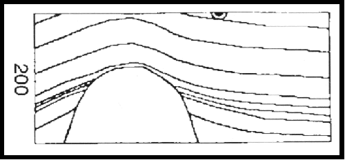