![]() Click to view article in PDF format.
Click to view article in PDF format.
GCSpectral Decomposition for Seismic Stratigraphic Patterns*
By
Kenny Laughlin1, Paul Garossino2, and Greg Partyka3
Search and Discovery Article #40096 (2003)
*Adapted for online presentation from the Geophysical Corner column in AAPG Explorer May, 2002, entitled “Spectral Decomp Applied to 3-D,” prepared by the authors. Appreciation is expressed to the authors, to R. Randy Ray, Chairman of the AAPG Geophysical Integration Committee, and to Larry Nation, AAPG Communications Director, for their support of this online version.
1Landmark Graphics, Denver; Col.orado
2Upstream Technology Group, BP, Houston, Texas
3Upstream Technology Group, BP, Sunbury, U.K.
While seismic processors have long used spectral decomposition, it is only in recent years that it has been applied directly to aspects of 3-D seismic data interpretation. The method for doing this was first published in “The Leading Edge” in 1999, in a paper by Greg Partyka et al., that illustrated the idea of using frequency to “tune-in” bed thickness.
Although spectral decomposition is a relatively new technique, some companies are experiencing great success in many basins around the world. (Most of the best examples are in clastic environments where depositional stratigraphy is a key driver.) Companies using spectral decomposition observe significant detail from these images at great depth – but have found that interpretation and integration with well data and models are critical to its success.
|
|
Click to view sequence highlighting different parts of reservoir (thicker to thinner).
As shown by the channel system in Figure 1, spectral decomposition can extract detailed stratigraphic patterns that help refine the geologic interpretation of the seismic. The concept behind spectral decomposition is that a reflection from a thin bed has a characteristic expression in the frequency domain that is indicative of temporal bed thickness. In other words, higher frequencies image thinner beds, and lower frequencies image thicker beds. This approach is similar to how remote sensing uses sub-bands of frequencies to map interference at the earth’s surface. Just like remote sensing, it is very important to dynamically observe the response of the reservoir to different frequency bands. The key is to create a set of data cubes or maps, each corresponding to a different spectral frequency, which can be viewed through animation to reveal spatial changes in stratigraphic thickness. Spectral decomposition reveals details that no single frequency attribute can match. Based on well-understood principals, typical amplitude maps are dominated by the frequency content of seismic data and will best image stratigraphy with thickness related to the dominant frequencies processed with the seismic. This is illustrated in Figure 2a, where we have a stratigraphic feature that varies in thickness. If the frequency content is high, thinner stratigraphic features will be “tuned” in and highlighted by higher amplitude (Figure 2b). If the frequency content is lower, thicker stratigraphic features will stand out (Figure 2c). What is needed is to see all the different stratigraphic thicknesses in a meaningful way. Spectral decomposition provides this by generating a series of maps or cubes that observe the response of the reservoir to different frequencies. These are then animated allowing the interpreter’s eye to catch subtle changes in the reservoir through motion. There are other good methods that can analyze tuning, but none are as easy to create or as routinely used as the method of animation called the “Tuning Cube.” To use spectral decomposition, you would interpret a seismic horizon and create a seismic amplitude map. The amplitude map is critical as a base to determine if spectral decomposition is adding to your interpretation. If you believe that amplitude is a meaningful indicator for reservoir presence, then spectral decomposition is a new step in the interpretation workflow. The seismic horizon is then used to transform a window of the data around the event of interest into the frequency domain and generate a series of amplitude maps at different frequencies. Thin bed interference will cause notches in the frequency domain related to the bed’s thickness. This is expressed on the amplitude maps as areas of high and low amplitude when animating through the different maps. Subtle changes in reservoir thickness or internal heterogeneities can be observed when comparing these images. Very quickly you will get a feel for areas with active stratigraphic variation that need to be evaluated in more detail. Tracking between these maps and the seismic cross-section is critical to determine if the features you are seeing are geologically meaningful. So is combining these images together. For example, Figure 3 contains a stratigraphic feature that appears to have a fan geometry. At lower frequencies from the “Tuning Cube,” the feeder channel of the “fan” is highlighted (Figure 3, left image). At higher frequencies, different lobes of the fan geometry are highlighted (Figure 3, middle image). At the highest frequencies available in the seismic data, the thinnest areas are highlighted (Figure 3, right image). In this example, there are actually 30 images that need to be animated to allow the eye to catch all of the detail available. Integration with well control is critical to determining the accuracy of the geologic interpretations. As mentioned, spectral decomposition is a relatively new technique that already has helped bring great success in many basins around the world. As such, it is poised to become an essential tool for the geologic interpretation of seismic data.
Partyka, G., J. Gridley, and J. Lopez, 1999, Interpretational applications of spectral decompositiion in reservoir characterization: The Leading Edge, v. 18, p. 353-360 |
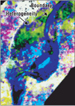 Figure 1– Spectral decomposition images
combined to highlight channel edges and thins as well as overbank
heterogeneity.
Figure 1– Spectral decomposition images
combined to highlight channel edges and thins as well as overbank
heterogeneity.