Figure Captions

	Figure 1. An inline from the 30 Hz voice component after spectral decomposition with spectral balancing and its amplitude spectrum. Notice the frequency width on both sides of the amplitude maxima seen at 30 Hz.
	Figure 2. (a) Segment of an inline through the input 3-D seismic amplitude and corresponding 65 Hz, (b) spectral magnitude, (c) spectral phase, and (d) spectra voice volumes. Notice the vertical discontinuities in the highlighted portion are poorly seen in the original broadband data; are not seen in the spectral magnitude component; but are clearly seen in the spectral phase and voice components. The voice component has the advantage in that it can easily be interpreted and processed (e.g. using coherence) as one would the original seismic amplitude data.
	Figure 3. An inline from the (a) input seismic data, and (b) input seismic data with spectral balancing. The amplitude spectra for both the datasets are shown in the insets to the lower right.
	Figure 4. (top row) Stratal slices 40 ms above the horizon close to 1700 ms, from the coherence attribute run on (a) input seismic data volume, (b) the input seismic volume with spectral enhancement, (c) voice component at 65 Hz, (d) voice component at 75 Hz, and (e) voice component at 85 Hz.
	Figure 5. (bottom row) Time slices at 1322 ms, from the coherence attribute run on (a) input seismic data volume, (b) the input seismic volume with spectral enhancement, (c) voice component at 65 Hz, (d) voice component at 75 Hz, and (e) voice component at 85 Hz.

Examples

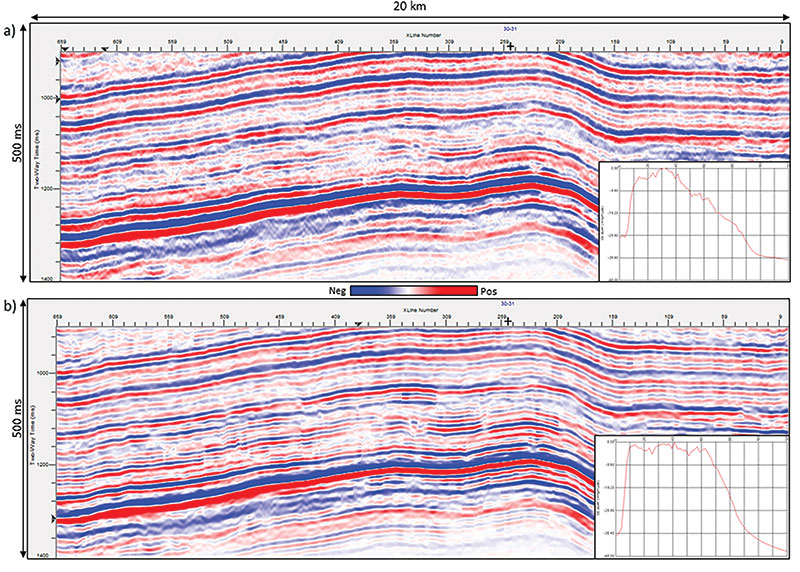
We show an example of a voice component section in Figure 1, along with its amplitude spectrum. Such voice components offer more information that could be processed and interpreted. We have focused on interpretational objectives of spectral decomposition in our earlier articles in the Geophysical Corner (Spectral Decomposition's Analytical Value – Search & Discovery Article #41260, and Extracting Information from Texture Attributes – Search & Discovery Article #41330) and demonstrated our examples pertaining to channels and other stratigraphic features. In this article our examples focus on faults and fractures.

In Figure 2 we show a segment of a seismic section from a 3-D seismic volume from northern-central Alberta, Canada. The equivalent sections from the spectral magnitude, phase component, and the voice component at 65 Hz are shown in Figures 2b, c and d respectively. Notice that the vertical discontinuity information is not clearly seen on the spectral magnitude, but rather on the phase component. The voice component combines both attributes and nicely delineates the discontinuities. This observation could be exploited to our advantage by either interpreting the discontinuity information as such, or by running a discontinuity attribute, such as coherence, on the voice component volume.

Traditionally, the spectral component magnitudes at different dominant frequencies have been utilized for obtaining detailed perspectives on stratigraphic objectives. As an example, the thickness of a channel is correlated with the spectral magnitude. More detailed information on seismic geomorphology can be gained by visualizing data at specific frequencies, or combining data with different frequencies using RGB color schemes. Another conclusion that one can have is that if the input data are spectrally balanced, or if its frequency bandwidth is somehow extended, the resulting volumes could lead to higher discontinuity detail. We focus on this aspect in this article.

Method

In another Geophysical Corner article (Spectral Balancing Can Enhance Vertical Resolution – Search & Discovery Article #41357), Marfurt and Matos described an amplitude-friendly method for spectrally balancing the seismic data. In this method, the data are first decomposed into time frequency spectral-components. The spectral magnitude is averaged over all the traces in the data volume spatially and in the given time window, which yields a smoothed average spectrum.

Next, the peak of the average power spectrum also is computed. Both the average spectral magnitude and the peak of the average power spectrum are used to design a single time-varying spectral balancing operator that is applied to each and every trace in the data. As a single scalar is applied to the data, the process is considered as being amplitude friendly.

Figure 3 shows segments of a seismic section and its equivalent section after spectral balancing. The individual amplitude spectral before and after are shown as insets. Notice that after spectral balancing the seismic section shows higher frequency content and the amplitude spectra is flattened.

Encouraged with the higher frequency content of the data, we run Energy Ratio coherence on the input data as well as the spectrally balanced version of the data. The results are shown in Figures 4a, b and 5a, b, where we notice the better definition of the NNW-SSE faults as well as the faults/fractures in the E-W direction on the coherence run on spectrally balanced version.

Finally, we run the spectral decomposition on spectrally balanced version of the input seismic data, and put the voice components through to Energy Ratio coherence computation. In Figures 4c, d, e and 5c, d, e we show time slices and horizon slices at different levels from the 65, 75 and 85 Hz frequency volumes. Notice the clarity in the definition of the discontinuities on both sets of displays. Such data lead to better interpretation of the discontinuities than carrying out the same exercise of the input data.

Conclusions

The conclusions that one can draw from the foregoing examples is that spectral balancing of seismic data, when performed in an amplitude-friendly way, leads to higher frequency content – which in turn exhibits detailed definition of faults and fractures. Such discontinuity information can be interpreted better on coherence displays in the zone of interest. Coherence attribute computation performed on spectral decomposition after spectral balancing, or on the voice components at higher frequencies yields higher detail with regard to the faults and fractures.

Return to top.