^GCAutotracking Horizons in Seismic Records*

Satinder Chopra¹ and Kurt J. Marfurt²

Search and Discovery Article #41489 (2014)
Posted November 17, 2014

*Adapted from the Geophysical Corner column, prepared by the authors, in AAPG Explorer, November, 2014, and entitled "Autotracking Your Way to Success". Editor of Geophysical Corner is Satinder Chopra ([email protected]). Managing Editor of AAPG Explorer is Vern Stefanic.

¹Arcis Seismic Solutions, TGS, Calgary, Canada ([email protected])
²University of Oklahoma, Norman, Oklahoma

General Statement

A horizon is a reflection surface picked on a 3-D seismic data volume that is considered to represent either a lithologic interface or a sequence stratigraphic boundary in the subsurface. Usually, an interpreter begins the exercise of identifying the different subsurface horizons by correlating the available well log data with the seismic data. In its simplest form, such identification can be done by hanging an impedance log curve on the seismic data – or more quantitatively, by generating a synthetic seismogram from the impedance log curve using an appropriate wavelet and correlating the result with measured seismic traces about the well. Depending on the seismic data quality and either the presence or lack of isolated strong reflectors, identifying horizons can be a trivial exercise or a challenging problem.

♦General statement
♦Figures
♦Metod
♦Examples
♦Conclusions

Figure Captions

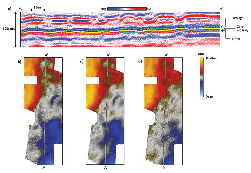
	Figure 1. (a) Vertical slice AA' through seismic amplitude showing three alternative horizon picks corresponding to autotracked troughs, zero-crossings (going from trough to peak), and peaks. Note how the yellow zero-crossing horizon pick is smoother. Corresponding time-structure maps computed from picks of (b) peaks, (c) zero-crossings, and (d) troughs. Note that (c) is less contaminated by noise. Data courtesy of Arcis Seismic Solutions, TGS.
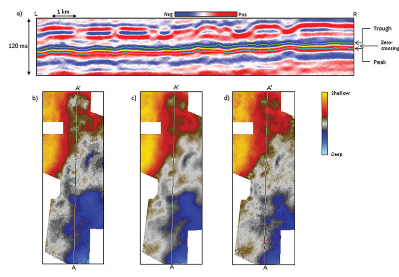	Figure 2. (a) Vertical slice AA' through seismic amplitude after structure-oriented median filtering showing three alternative horizon picks corresponding to autotracked troughs, zero-crossings (going from trough to peak), and peaks. Corresponding time-structure maps computed from picks of (b) peaks, (c) zero-crossings, and (d) troughs. All three time-structure maps exhibit less noise, though (b) and (d) exhibit a "patchy" appearance common to median filters. Data courtesy of Arcis Seismic Solutions, TGS.
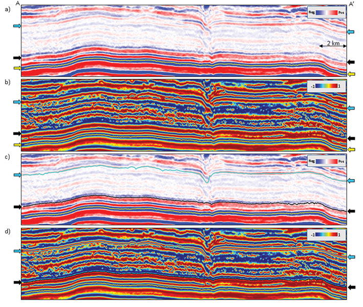	Figure 3. Segment of a seismic section (crossline) through (a) the input seismic volume after median filtering, and (b) the equivalent section through the cosine of instantaneous phase attribute. The prominent horizon in yellow was autotracked on the blue trough and is shown on both sections. The zero-crossing at the location of the black arrows and the peak at the location of the cyan arrows cannot be successfully autotracked. In contrast, autotracking works well for these horizons on the cosine of instantaneous phase attribute shown in (d) and then overlaid on the seismic shown in (c). They seem to fit perfectly.
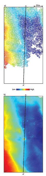
	Figure 4. Autotracking attempted on seismic data on the zero-crossing horizon indicated by the black arrows on Figure 3. The lower part of the horizon was not successfully tracked. Similar autotracking attempted on cosine of instantaneous phase attribute tracks the horizon completely. Data courtesy of Arcis Seismic Solutions, TGS.

Method

In the beginning, horizons were handpicked, posted on a map and hand-contoured. In the 1970s and 1980s the hand picks were manually digitized by a technician, loaded into a database and then contoured using a mainframe computer. Removing bad picks from the database required extra requests. Such a task was laborious, inefficient and usually not very accurate. With the introduction of the workstations, this task became automated – much to the relief of the seismic interpreters.

Today's automated horizon-picking algorithms are much more sophisticated than those of a decade ago. While automated pickers appear to simply find peaks, troughs and zero-crossings on adjacent traces, internally there are constraints of correlation coefficient, dip and coherence that provide the ability to pick through moderate quality data with relatively complicated waveforms. Nevertheless, autotracking is sensitive to the variations in the signal-to-noise (S/N) ratio of the seismic data:

High S/N ratio of data implies locally smooth and continuous phase of the reflections to be picked, and usually yields a good autotracked surface.
Data with low S/N ratio implies no smoothness or consistency in the phase to be tracked and prevents reliable horizon picking.

Autotracking works very well on coherent seismic reflectors. With a single click of a cursor on the given phase (peak, trough, and positive to negative or negative to positive zero crossings) the complete surface can be rapidly picked in no time. Through the use of time-structure and dip magnitude maps, one can just as rapidly identify busts in the picking algorithm that may need to be interactively repaired. Almost as important as autopicking, most software packages provide an autoerasing option, which removes either the last one or two steps or provides erasure within user defined polygons.

Because of lateral changes in overburden and vertical changes in reflectivity, seismic data quality often varies laterally and vertically. While 3-D autopickers may work on strong, isolated reflectors, they may work poorly at the target of interest. In such cases, the interpreter manually or semi-automatically picks a grid of every 10^th or 20^th inline and crossline. With this extra guidance, the autotracker will work for much if not most of the survey.

Examples

A question that usually arises is: Why should one pick a zero-crossing if the seismic well tie is a peak or a trough? If the objective is to map an abrupt change in impedance between thick layers, the well tie usually will be a peak or a trough.

If the objective is to map a thin bed, the well tie is usually a zero-crossing. Our experience has shown that seismic travel time picks are less contaminated with noise along a zero-crossing than along a peak or a trough. Peaks and troughs are locally flat, so a small amount of noise shifts them vertically. In contrast, zero-crossing occurs where the amplitude changes most rapidly, such that its location is less impacted by low amplitude noise. Of course, the quality of such horizon displays will depend on the S/N ratio of the data, which certainly can be improved by using structure-oriented filtering or median filtering (see October 2014 Geophysical Corner – Search and Discovery Article #41476).

In Figure 1 we show a vertical slice through a seismic amplitude volume with automatic picks made of peaks (in cyan), troughs (in green), and zero-crossings (in yellow). Notice the resulting time-structure maps from the peak and trough picks are noisier than that from the zero-crossing picks. As the input seismic data has random noise on it as it was not conditioned before picking, each of the horizon displays has a jittery appearance.

In Figure 2, we show the equivalent segment of the seismic section shown in Figure 1, but after application of a structure-oriented median filter. The same horizons are again picked and mapped as before. Notice the cleaner look of the seismic section as well as three horizon displays. Needless to mention, horizon-based dip magnitude, dip azimuth and curvature will show even greater improvements.

The take-away from this simple exercise is that horizons could be picked along zero-crossings in preference to peaks or troughs. If the well tie is to a peak or trough, one simply computes the quadrature (also called the Hilbert transform and the imaginary part) of the seismic data, which converts peaks and troughs to -/+ and +/- zero-crossings.

Not all geological markers of interest may correspond to a strong peak or a strong trough. Many times a horizon has to be tracked along a weak amplitude peak or trough, where autotracking breaks down. In such cases the use of seismic attributes has been suggested.

In the November 2004 Geophysical Corner – Search and Discovery Article #40141, an interesting application in terms of the use of the cosine of instantaneous phase attribute for autotracking was discussed. The complex trace attributes serve to examine the amplitude, phase and frequency delinked from each other. The instantaneous phase attribute can be analyzed without the amplitude information, but is discontinuous for both 180 degrees and -180 degrees. The cosine of instantaneous phase has a value of unity for both these angles, and so is a better attribute to pick horizons on.

In Figure 3a we show a segment of a seismic section, where a strong trough (yellow arrows) has been conveniently autotracked. However, if the zero-crossing corresponding to the blue and black arrows has to be picked, it does not track well.

The equivalent cosine of instantaneous phase attribute section is shown in Figure 3b. Horizons are tracked corresponding to the zero-crossings along the blue and black arrows on this data volume (Figure 3d) and overlaid on the seismic as shown in Figure 3c. Both the horizons appear to be tracked well.

In Figure 4a we show the display of the autotracked horizon attempted on the seismic corresponding to the black arrow. Notice it is not tracked as a complete surface. The same horizon when tracked on the cosine of the instantaneous phase attribute is shown in Figure 4b and is seen as a complete, relatively smooth surface.

Most autotrackers internally use a cross-correlation algorithm to compare adjacent waveforms. Weak reflectors can be overpowered by adjacent stronger reflectors as well as by stronger cross-cutting noise. By balancing the amplitude, the cosine of instantaneous phase attribute minimizes these interference effects.

Conclusions

If horizons are autotracked along zero-crossings on 3-D seismic traces, they yield smoother surfaces than those picked on peaks or troughs. One therefore can obtain more accurate surfaces by picking zero-crossings on the corresponding quadrature of the original data volume. Structure-oriented filtering applied to the amplitude data results in less noisy time-structure maps. In the case of weak reflectors, the application of the cosine of instantaneous phase attribute can help commercial autotrackers perform better.