![]() Click to view article in PDF format.
Click to view article in PDF format.
GC![]() Phase
Phase![]() Residules Can Help Define Channels*
Residules Can Help Define Channels*
Marcilio Matos1,2 and Kurt J. Marfurt2
Search and Discovery Article #41140 (2013)
Posted June 30, 2013
*Adapted from the Geophysical Corner column, prepared by the author, in AAPG Explorer, March, 2013, and entitled “Out of ![]() Phase
Phase![]() Doesn’t Mean Out of Luck”.
Doesn’t Mean Out of Luck”.
Editor of Geophysical Corner is Satinder Chopra ([email protected]). Managing Editor of AAPG Explorer is Vern Stefanic
1Signal Processing Research, Training and Consulting, Norman, Oklahoma ([email protected])
2University of Oklahoma, Norman, Oklahoma
Interpreters use ![]() phase
phase![]() each time they design a wavelet to tie seismic data to a well log synthetic. A 0-degree
each time they design a wavelet to tie seismic data to a well log synthetic. A 0-degree ![]() phase
phase![]() wavelet is symmetric with a positive peak, while a 180-degree
wavelet is symmetric with a positive peak, while a 180-degree ![]() phase
phase![]() wavelet is symmetric with a negative trough. Given a 0-degree
wavelet is symmetric with a negative trough. Given a 0-degree ![]() phase
phase![]() source wavelet, thin beds give rise to ±90-degree
source wavelet, thin beds give rise to ±90-degree ![]() phase
phase![]() wavelets.
wavelets.
Mathematicians define ![]() phase
phase![]() using a “complex” trace, which is simply a pair of traces:
using a “complex” trace, which is simply a pair of traces:
1) The first trace is the measured seismic data, and forms the “real” part of the complex trace.
2) The second trace is the ![]() Hilbert
Hilbert![]()
![]() transform
transform![]() of the measured data, and forms the imaginary part of the complex trace.
of the measured data, and forms the imaginary part of the complex trace.
Note in Figure 1a that when the real part of the trace is positive, the imaginary part is a minus-to-plus zero crossing. In contrast, when the real part of the data is a minus-to-plus zero crossing, the ![]() Hilbert
Hilbert![]()
![]() transform
transform![]() is a trough. This latter phenomenon allows us to use the “instantaneous”
is a trough. This latter phenomenon allows us to use the “instantaneous” ![]() Hilbert
Hilbert![]()
![]() transform
transform![]() to generate an amplitude map of a thin bed that was previously picked on the well log as zero crossing of the measured (or real) data.
to generate an amplitude map of a thin bed that was previously picked on the well log as zero crossing of the measured (or real) data.
Now let’s map both parts of the complex trace on the same plot. As you may remember from high school algebra, the real part is plotted against the x-axis and the imaginary part against the y-axis. We plot the same 100 ms (50 samples) of data “parametrically” on the complex plane.
Note in Figure 1b that the waveform progresses counterclockwise from sample to sample. We map this progression using the ![]() phase
phase![]() between the imaginary and real parts. If we use the arctangent to compute the
between the imaginary and real parts. If we use the arctangent to compute the ![]() phase
phase![]() , we encounter a 360-degree discontinuity each time we cross ±180 degrees (Figure 1c). Note how peaks and troughs in
Figure 1a appear at 0 degrees and ±180 degrees in
Figure 1c.
, we encounter a 360-degree discontinuity each time we cross ±180 degrees (Figure 1c). Note how peaks and troughs in
Figure 1a appear at 0 degrees and ±180 degrees in
Figure 1c.
Now, if we computed the ![]() phase
phase![]() by hand, we would obtain the much more continuous
by hand, we would obtain the much more continuous ![]() phase
phase![]() shown in
Figure1d, which is an “unwrapped” version of
Figure 1c, and in this unwrapped image, note there is still a discontinuity at t=850 ms; however, this discontinuity is associated with waveform interference (geology) and not mathematics. Such discontinuities form the basis of the “thin-bed indicator” instantaneous attribute introduced 30 years ago.
shown in
Figure1d, which is an “unwrapped” version of
Figure 1c, and in this unwrapped image, note there is still a discontinuity at t=850 ms; however, this discontinuity is associated with waveform interference (geology) and not mathematics. Such discontinuities form the basis of the “thin-bed indicator” instantaneous attribute introduced 30 years ago.
The above discussion illustrates the concept of ![]() phase
phase![]() unwrapping and discontinuities based on the complex trace used in instantaneous attributes. A more precise analysis can be obtained by applying the same process to spectral components of the seismic data. Spectral decomposition is a well-established interpretation technique. The seismic data are decomposed into a suite of spectral components, say at intervals of five Hz.
unwrapping and discontinuities based on the complex trace used in instantaneous attributes. A more precise analysis can be obtained by applying the same process to spectral components of the seismic data. Spectral decomposition is a well-established interpretation technique. The seismic data are decomposed into a suite of spectral components, say at intervals of five Hz.
Most commonly we use spectral magnitude components to map thin bed tuning, while some workers use them to estimate seismic attenuation, 1/Q. The ![]() phase
phase![]() components are less commonly used, but often delineate subtle faults. Here, we will show how the identification of discontinuities in the unwrapped instantaneous
components are less commonly used, but often delineate subtle faults. Here, we will show how the identification of discontinuities in the unwrapped instantaneous ![]() phase
phase![]() discussed above can be extended to unwrapped
discussed above can be extended to unwrapped ![]() phase
phase![]() of spectral components.
of spectral components.
|
|
Let us illustrate the use of such discontinuities by applying them to the well-studied Stratton Field data volume acquired over a south Texas fluvial-deltaic system by the University of Texas Bureau of Economic Geology. In our Stratton Field example, thin channels give rise to tuning effects and subtle amplitude anomalies as shown in
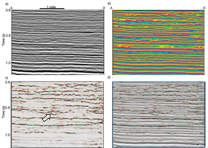
Figure 2a. While we can detect the channel system on time and horizon slices, they are difficult to see on vertical slices through the seismic amplitude data (Figure 3a). Determining the thickness of the channel on the seismic amplitude image is even more difficult. The corresponding slice through the instantaneous
One approach to improving this image is to unwrap the instantaneous
Figure 3c shows this computation, where the hue component of color corresponds to the frequency of the discontinuity and the intensity or brightness to its strength. A block arrow clearly delineates the top and bottom of the channel.
Figure 3d co-renders the Thin meandering channels are often visible on amplitude time slices (Figure 2). |
 General statement