![]() Click to view article in PDF format.
Click to view article in PDF format.
GCAn '![]() Elastic
Elastic![]()
![]() Impedance
Impedance![]() ' Approach*
' Approach*
Satinder Chopra1and Ritesh Kumar Sharma1
Search and Discovery Article #41082 (2012)
Posted November 12, 2012
*Adapted from the Geophysical Corner column, prepared by the author, in AAPG Explorer, October, 2012. Editor of Geophysical Corner is Satinder Chopra ([email protected]). Managing Editor of AAPG Explorer is Vern Stefanic; Larry Nation is Communications Director. AAPG©2012
1 Arcis Corp., Calgary, Canada ([email protected])
A detailed investigation of seismic amplitudes can yield information pertaining to lithological variation in subsurface sedimentary rock formations and the existence and extent of some hydrocarbon zones. This objective can be facilitated in a process called seismic inversion, which transforms seismic amplitudes into acoustic ![]() impedance
impedance![]() values. In doing so, the seismic reflection response gets transformed into layered
values. In doing so, the seismic reflection response gets transformed into layered ![]() impedance
impedance![]() response, which makes the interpretation of the lithological and fluid information more convenient – each transformed
response, which makes the interpretation of the lithological and fluid information more convenient – each transformed ![]() impedance
impedance![]() trace can now be considered as an
trace can now be considered as an ![]() impedance
impedance![]() log curve and the seismic volume as logs recorded in wells drilled at every seismic trace location. Just as the changes in the character of
log curve and the seismic volume as logs recorded in wells drilled at every seismic trace location. Just as the changes in the character of ![]() impedance
impedance![]() log curves are indicative of changes in lithology, porosity and fluid content, similar changes seen on inverted
log curves are indicative of changes in lithology, porosity and fluid content, similar changes seen on inverted ![]() impedance
impedance![]() traces are interpretable of these properties in a lateral sense over an area and so over a volume.
traces are interpretable of these properties in a lateral sense over an area and so over a volume.
Acoustic ![]() impedance
impedance![]() inversion has now become an integral part of most interpretation projects today. While this is a beneficial tool for the seismic interpreter, acoustic
inversion has now become an integral part of most interpretation projects today. While this is a beneficial tool for the seismic interpreter, acoustic ![]() impedance
impedance![]() inversion is usually run on stacked seismic traces – that is, the individual prestack time migrated offset gathers are stacked and then transformed into
inversion is usually run on stacked seismic traces – that is, the individual prestack time migrated offset gathers are stacked and then transformed into ![]() impedance
impedance![]() . To better exploit the fluid effects that manifest on prestack gathers as variation of amplitudes with offset or angle, prestack
. To better exploit the fluid effects that manifest on prestack gathers as variation of amplitudes with offset or angle, prestack ![]() impedance
impedance![]() inversion also can be carried out. Of course, it would take longer - and so the trade-off is usually between the cost, time and the method to be used.
inversion also can be carried out. Of course, it would take longer - and so the trade-off is usually between the cost, time and the method to be used.
|
|
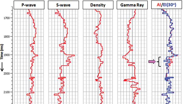
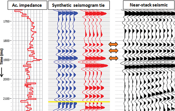
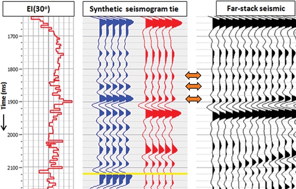
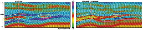
A simple way to examine the variations of amplitude as a function of offset is to generate the offset-limited seismic volumes, such as the near-, mid- and far-offset (or angle) volumes. Variations seen on these volumes in desired zones could then be indicative of the fluid information. For example, a low- As amplitudes of the near-offset traces are related to the changes in acoustic Back in 1999, Patrick Connolly from BP pointed this out and suggested the generalization of acoustic The In actual practice, the CMP gather at the position of the well is picked up, different angle ranges are selected and angle stacks generated. Given the VP, VS and density log curves, the Another useful and meaningful display is the comparison of the acoustic The gas was detected during mud logging and on the electric log curve; however, the density and neutron curve crossover is not as high as expected, probably due to low saturation as well as its position. The saturation is expected to increase in the up-dip direction. Notice that there is a decrease of It may be mentioned that the As stated, In Figure 2 we show the correlation of a synthetic seismogram (generated with the acoustic In Figure 4 we show a comparison of a segment of an acoustic Thus We thank PetroNorte, Colombia, for giving us permission for presentation of the results shown in this study. We also thank Arcis Seismic Solutions for permission to present this work. |
 General statement