![]() Click to view article in PDF format.
Click to view article in PDF format.
PSFrom collection to utilization: Outcrop analog data in a 3D world*
By
John B. Thurmond1
Search and Discovery Article #40126 (2004)
*Adapted from poster presentation at AAPG Annual Meeting, Dallas, Texas, April 18-21, 2004.
1University of Texas at Dallas ([email protected])
The collection of three-dimensional data from outcrops is playing an increasingly important role in reservoir characterization studies. There are a variety of techniques that can be used to acquire three-dimensional data from outcrops, and each should be applied individually or in concert to collect data in specific circumstances. The current suite of emerging methods typically used in outcrop-scale measurement includes traditional surveying, direct GPS measurement, laser scanning (LIDAR), photogrammetry, and photorealistic mapping (texture draped geometry). Depending on the morphology, setting, and particular data needs of a specific outcrop, different methods can be used to acquire data. Case studies of individual outcrops will be shown to illustrate the problems and benefits of several of these methods.
Once three-dimensional data is collected, utilizing the data can present its own set of challenges. Each collection method produces a different type of data, each of which requires a variety of processing and interpretation methods to utilize effectively. In most cases, there is also the need to integrate data from a variety of sources into a single interpretable data set. Again, case studies provide specific illustrations of effective methods that have been used in various projects to produce reservoir models from a variety of environments, including deep-water channel systems, heavily faulted fluvial environments, and carbonate build-ups.
|
uAbstractuPhotorealistic outcrop capture
uAbstractuPhotorealistic outcrop capture
uAbstractuPhotorealistic outcrop capture
uAbstractuPhotorealistic outcrop capture
uAbstractuPhotorealistic outcrop capture
uAbstractuPhotorealistic outcrop capture
|
Figure Captions
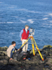
MethodsGPS Mapping (Figures 1 and 4) The most straightforward method for mapping geologic surfaces in 3D is to simply walk them out with a high-precision GPS system. This type of mapping is most appropriate on accessible outcrops and in places where contacts or facies boundaries are subtle. Normally, Real-Time Kinematic GPS systems are used, which provide an accuracy of approximately 2cm. Due to the practicalities of efficiently walking on a geologic surface, the normal accuracy is about 50 cm.
Advantages: High accuracy (50 cm or less). Accurate data distribution (no surface, no data) eliminates “interpolation” problems.
Disadvantages: Slow (5-10 km per day). Re-interpretation can require re-mapping.
Laser Rangefinder Mapping (Figures 2 and 3) Often, it is not physically possible to “walk” on a stratigraphic surface, so other techniques are required. Reflectorless Laser Rangefinders, coupled with high-precision GPS receivers, provide the opportunity to capture data from such locations. These systems integrate an EDM for distance measurement with a digital compass and inclinometer, so 3D position can be measured remotely. However, this technique requires surfaces that are visible from a remote location.
Advantages: Fast.
Disadvantages: Lower accuracy (varies with distance). Encourages interpolation/extrapolation. Re-interpretation can require re-mapping.
Photorealistic Outcrop Capture (Figures 7 and 8) Using a scanning laser system, coupled with a high-accuracy GPS system, it is possible to scan the topography of an outcrop with a high degree of accuracy. Digital photographs can then be accurately mapped to the topography, which provides an accurate, three-dimensional model of the outcrop. This model can then be interpreted in 2D (on the photographs) or in 3D (on the model), and re-interpreted as often as necessary. Some laser systems provide the capability of scanning color simultaneously with distance, but the data sets are incredibly difficult to work with, even with the most advanced 3D workstations available. However, 3D geometry combined with texture data from photographs renders extremely quickly, even on laptops (ask for a demo!).
Advantages: Fast. High accuracy (5-10cm pixel error (!)). Provides images with data, so interpretations are believable. Data sets can be re-interpreted as paradigms change.
Disadvantages: Expensive equipment required. Processing can be intensive.
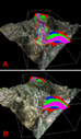
CarbonatesLocation: Last Chance Canyon, Guadalupe Mountains, New Mexico (Figures 5 and 6) Problem: Excellent 3D exposures of a mixed carbonate and siliciclastic system. Antecedent topography is an important control on subsequent facies deposition. Mapping of paleogeomorphological surfaces and subsequent facies in 3D provides the opportunity to build models which predict facies deposition as a function of topography for specific systems. Techniques: Currently, only GPS mapping has been applied. Photorealistic mapping scheduled for Q2 of 2004. Sample transects integrated into a 3D VRML data base containing outcrop photos, photomicrographs and sample descriptions (the live visualization has been demonstrated at oral and poster presentations). Results: Current: 3D geologic model of (hydrodynamic?) mud-mounds. Model provides evidence for re-interpretation of processes controlling mud-mound deposition. Future: Interpreted photorealistic model of Last Chance Canyon. This will provide a framework for building a 3D geologic model of the canyon, which will be an excellent research and teaching data set.
SiliciclasticsLocation: Eocene Ainsa II deepwater channel and lobe complex of the South-Pyrenean Foreland Basin, Spain (Figures 7, 8, 9, 10, and 11) With: Ole J. Martinsen and Tore M. Løseth, Jan Rivenaes, and Kristian Soegaard, Norsk Hydro Research Centre Problem: These deep-water siliciclastics are an excellent analog for active production fields in offshore Angola. Accurate 3D data captured from outcrop facies relationships is used to build a reservoir model, which can help predict heterogeneity in the subsurface and will also make an excellent teaching data set. Techniques: Numerous integrated photorealistic models were used to collect accurate 3D representations of the outcrop. Surfaces were interpreted in an immersive visualization environment (a CAVE) and, combined with spatially accurate 3D structural models, produced by the University of Barcelona. Results: A reservoir model was produced from the 3D data acquired from the outcrops.
Fault MappingLocation: Various faults in central Utah (Figures 12 and 13) With: Rod Myers, Peter Vrolijk, and Tom Hauge, ExxonMobil Upstream Research Problem: Fault systems have complicated 3D geometries, and fault properties vary as a function of geometry. Mapping of fault geometries and properties in 3D allows these relationships to be determined quantitatively, allowing them to be applied algorithmically to fault geometries observed in the subsurface. Techniques: Many of these faults are difficult to see from a distance, and outcrops are generally accessible, so direct GPS mapping was used to collect data. Individual faults and stratigraphic surfaces were walked out, and the intersection of topography and the surfaces was sufficient to produce a 3D model. Results: A faulted framework model was produced in gOcad using the 3D data collected in the field. This model will be used to visualize fault properties as a function of geometry.
AcknowledgmentsThe author would like to thank the following individuals and companies for financial, conceptual, and/or fieldwork support for these projects: Norsk Hydro Research Centre ExxonMobil Upstream Research NSF Graduate Fellowship Carlos Aiken Xueming Xu Janok Bhattacharya
The author thanks Roxar for the generous donation of their software to UTD. |


