Online Journal for E&amp;P Geoscientists

uHistory of Long Beach Unit

uHistory of Long Beach Unit

uHistory of Long Beach Unit

uHistory of Long Beach Unit

uHistory of Long Beach Unit

uHistory of Long Beach Unit

uHistory of Long Beach Unit

uHistory of Long Beach Unit

uHistory of Long Beach Unit

uHistory of Long Beach Unit

uHistory of Long Beach Unit

uHistory of Long Beach Unit

uHistory of Long Beach Unit

uHistory of Long Beach Unit

uHistory of Long Beach Unit

uHistory of Long Beach Unit

Figure 1. Location map showing oil fields in the Los Angeles Basin of southern California, with the Wilmington oil field shown in light gray.

uConclusions

uAcknowledgments

uReferences

Figure Captions (1-2)

Figure 2. Map of the Long Beach area showing the areas of the Wilmington oil field where Tidelands Oil Production Company (western portion) and THUMS Long Beach Company (Long Beach Unit) are the field contractors. The city of Long Beach, Department of Oil Properties, operates both portions. The limits of the Wilmington field, along with those of the Long Beach field and the Seal Beach field, are shown. The coastline, harbor areas, breakwater, and oil-drilling islands are shown for reference. Pacific Energy Resources operates the polygonal area between the properties. The western notch is the Wilmington Townlot Unit (WTU), which is operated by Magness Petroleum Company. Exxon operates the southeast area (not delineated) as State Lease 186 Belmont Offshore. This portion is under abandonment.

Background

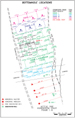
The Wilmington oil field of southern California (Figure 1), the largest oil field in the Los Angeles Basin (Biddle, 1991), has produced more than 2.6 billion barrels of oil (California Department of Conservation, 1999). Discovered in 1932, it produces from semi- and unconsolidated Pliocene and Miocene clastic slope and basin turbidite sandstones (Henderson, 1987; Blake, 1991). The individual reservoirs are defined by graded sequences of sandstone interlayered with siltstones and shales (Slatt et al., 1993). The entire sequence is folded and faulted (Mayuga, 1970; Clarke, 1987; Wright, 1991). Even the typical rhythmically deposited sequences have lenticular, lobate shapes and are complicated by basal scour, amalgamation, onlapping, and channeling. The result is a sequence of rocks that often appears to be uniform but is not. These complexities also result in permeability variations that hinder the producibility of the sandstones, impact waterflooding, and result in a substantial amount of bypassed oil.

The Wilmington field has been divided stratigraphically into seven producing zones, 52 subzones and, locally, into even finer subsubzones (Henderson, 1987). A serious effort was made to establish stratigraphic continuity in detail as fine as possible. The finer subdivisions are defined as hydrologic bodies or depositional sequences. Many techniques and tools were applied to characterize the thinner sand bodies into unique units, including core description combined with log-rock typing, detailed log correlation, production/injection history matching, bypassed pay-saturation analysis on recent pass-through wells, and reservoir simulation (Otott, 1996; Davies and Vessell, 1997; Davies et al., 1997). Six geologists spent the better part of one year working with thousands of old logs and assorted base maps to sort out a consistent and logical stratigraphic sequence. In addition to the authors, Keith Jones, Mike Henry, Linji An, Rick Strehle, and David K. Davies performed a significant portion of the characterization.

Although we are still learning about the intricacies of Wilmington field’s reservoirs, today’s computerized visualization tools, combined with advanced measurement-while-drilling (MWD) data, have contributed significantly to the collective knowledge base about this field. We thus confidently conclude that the field’s poorly drained sandstones remain ideal targets for horizontal drilling.

History of the Long Beach Unit

The Wilmington oil field is a faulted asymmetrical anticline. The reservoirs of the 10 larger fault blocks in the field have been managed independently. The city of Long Beach, Department of Oil Properties, operates most of them (Figure 2). The Wilmington Townlot Unit (WTU), a portion of the westernmost Fault Block I, is operated by Magness Petroleum Company. Pacific Energy Resources operates a portion of Fault Block II. Tidelands Oil Production Company is the field contractor for most of the western portion (Fault Blocks I–V). THUMS Long Beach Company is the field contractor for the eastern part of Wilmington oil field (Fault Blocks VI–90N), which is called the Long Beach Unit (LBU). The LBU was originally produced with more than 1000 wells drilled between 1965 and 1982 (Otott and Clarke, 1996). Despite the very long completion intervals used and water injection for pressure support, oil remained in pockets of tight, thin sandstones, as well as in areas with poor injection support. Widely ranging permeabilities and faulting caused typically viscous oil (12.5° to 16° API) to be left behind in sandstone units 6 to 15 m thick.

An additional 460 wells were drilled in the Long Beach Unit from 1982 to 1986 using a subzone approach to improve sweep efficiency, which allowed another 25.4 million cubic meters (m³), or 160 million barrels (bbl), to be produced. After 1986, bypassed sandstones were selectively perforated in even finer intervals. The first horizontal well was completed in November 1993 as part of the optimized waterflood project. Thirty-nine more horizontal wells have been drilled since then, using a combination of computerized mapping and digitized injection surveys to identify the dominant, unswept flow units. Reservoir exploitation was enhanced by geosteering supported by logging while drilling (LWD) and real-time analysis of MWD/LWD data to update cross sections.

Typically, the wells were placed 3 to 5 m (10 to 15 ft) below the top of the sandstone. Initial oil-production rates from the best horizontal wells exceeded 95.4 m³/day (600 bbl/day) and about 47.7 m³/day (300 bbl/day) from the average wells, at 80% water cut, stabilizing at about 15.9 m³/day after 300 days. Total unit oil production is 6042 m³/day (38,000 bbl/day). Blesener and Henderson (1996) describe several of the new engineering technologies that have been applied to the Long Beach Unit. These include coiled-tubing drilling, drill-cuttings injection, and reclaimed-water injection. In 1995, the LBU ran a 3-D seismic survey to help define the subsurface in greater detail (Otott et al., 1996). The survey did not provide the desired results, but it did serve as a valuable tool for deep work. Several exploratory prospects were identified. One or more of these may be drilled in 2003.

THUMS was purchased from ARCO by Occidental Oil and Gas Corporation in May 2000. In 2002, THUMS conducted a 3-D vertical seismic profile (VSP) in the area between Islands Freeman and Chaffee. These data are being processed.

History of the Old Wilmington Area

The history of the Wilmington oil field has been detailed by Mayuga (1970), Ames (1987), and Otott and Clarke (1996). More than 5000 wells have been drilled conventionally in the 70 years Old Wilmington has been on production. The entire field is on secondary recovery, and oil production is down to 1113 m³/day (7000 bbl/day) with an average water cut of 96.9%. Because of the steep, 14%-per-year decline, it was decided to investigate new ways to produce more oil. As part of this effort, Tidelands Oil Production Company has drilled 14 horizontal wells since 1993 in four heavily drilled (3000-plus wells) fault blocks (Phillips and Clarke, 1998; Phillips et al., 1998). The first horizontal well project was a “Huff ’n’ Puff ” conducted in 1993 in Fault Block I Tar zone. Two 274.3 m- (900 ft-) long horizontal wells were drilled into the D₁ sandstone. The second project was a steamflood in Fault Block II Tar zone. In 1995 for project 2, four horizontal wells were drilled on average 488 m (1600 ft) within the D₁ sandstone. A Fault Block IV Terminal zone waterflood well was drilled 335.3 m (1100 ft) within the Hxb sandstone in 1995 as the third project. Again in 1995, five horizontal wells were drilled into the Fault Block V Tar zone as part of a steamflood. The wells were drilled on average 457.2-m (1500 ft) horizontally within the S₄ sandstone. In 1997, a 304.8-m (1000-ft) horizontal well was drilled into the Hx₀ sandstone of Fault Block V Terminal zone to complete the fifth project.

For each project, the horizontal laterals for the waterflood wells were placed at the top of the sandstone to recover attic reserves. The laterals for the steamflood wells were placed at the bottom of the sandstone to maximize capture of oil through steam-assisted gravity drainage.

Except for the first project, 3-D modeling and visualization were used from planning through completion. To be effective, horizontal wells require precision placement. The studied areas required significant geologic evaluation and characterization. The area then was modeled with software that provided 3-D visual displays of stratigraphic and structural relationships and enabled excellent error checking of data and grids in 3-D space. The geologic model was revised and modified in 3-D space. The 3-D model provided a visual reference for well planning and communicating the spatial relationships contained within the reservoir. Accurate 2-D and 3-D visualization was used for interpreting the LWD response and monitoring well progress while drilling. Maps and section plots brought to the rig site allowed the drilling team to relate to the geology, thus providing a strong confidence factor. Accurate and rapid postdrilling analysis for completion-interval selection and LWD analysis completed the process.

Figure Caption (3)

Figure 3. Aerial photograph of Long Beach/Los Angeles Harbor showing the location of the three horizontal-well projects. North is to the top. On the left (west) is the steamflood project (case history 1) with four horizontal wells placed in the Tar zone below Terminal Island. The location of cross section A-B is shown. Case history 2 consists of five horizontal wells that cross under the Los Angeles River channel and are part of a Tar zone steamflood project in Fault Block V (FB V). The location of cross section CD is shown. Case history 3 involves a tight-radius horizontal well that lies stratigraphically below case history 2 in Fault Block V in the upper Terminal zone. Oil activities coexist with the busiest harbor in the country, and the Fault Block V steamflood is below Long Beach’s new $180 million aquarium.

Case Histories

Three case histories are presented herein. Case history 1 describes a thermal-enhanced recovery project that expanded on an existing steamflood project. The expansion area was subjected to detailed characterization with 3-D modeling and visualization before completion of the development project. The technologies developed in the steamflood project were applied to the areas in Fault Block V and are described as case histories 2 and 3. Figure 3 shows the location of the three case histories.

Figure Captions (4-12)

	Figure 4. Map of Fault Block II area showing the location of the Wilmington oil field Tar zone, Fault Block II-A steamflood project. Each phase of the project is shown in color code. The project described here focuses on the southern area where the four horizontal wells were drilled. Cross section A-B follows the well course of UP955.
	Figure 5. Type logs for Tar zone, Fault Block II (Well 2AU 30B 1). Original markers are shown in black, and the newly picked markers in red. The inset shows the T4 channel from well 2AT58B. Note the good saturation between D₁ and D_1E. The location of these two wells is shown in Figure 10.
	Figure 6. Map showing location of Fault Block II horizontal wells in relation to the subsidence bowl. Red contour lines are total elevation loss in feet. The four horizontal wells were completed in an area of 14 to 22 ft (4.3 to 6.7 m) of subsidence. Producing well courses are shown in blue, and steam-injection well courses are shown in green. The line of cross section A-B parallels well UP 955.
	Figure 7. Three components of subsidence correction. (A) Adjustments must be made for rock compaction that occurs after a well is drilled. (B) The kelly bushing must be corrected for subsidence that occurred prior to drilling. (C) Finally, an adjustment must be made within the formation to correct the overlying sediments for compaction that has occurred below.
	Figure 8. Structure map of the T marker in Fault Block IIA. Observation and horizontal wells are shown. Contour intervals shown are 50 ft (15.2 m) from –2400 to –3400 ft (–731.5 to –1036 m) below sea level.
	Figure 9. Cross section A-B, which follows the well course of UP 955. Perforations are shown on well course. The onlap of the D_1E is shown; no detail below EV is shown. The section is scaled in feet and has a 2x vertical exaggeration. The locations of the cross section and well UP 955 are also shown in Figures 3, 4, 6, and 8.
	Figure 10. Three-dimensional structural display of the T2 horizon in Fault Block II (FB II), showing locations of the two type wells in Figure 5. The T4 paleochannel cuts through several horizons.
	Figure 11. Three-dimensional display of the D_1F onlap onto the D₂ shale in Fault Block II. The figure has a 2x vertical exaggeration, and the units displayed are in feet.
	Figure 12. Three-dimensional display of Fault Block II showing locations of wells drilled for the steamflood project. The figure has a 2x vertical exaggeration, and the wellbores are greatly exaggerated to enhance the visual impact of the well pattern.

Case History 1: Fault Block II, Tar Zone Steamflood Project

Case history 1 is in the Tar zone of Fault Block II (Figure 4). The Tar zone of the lower Pliocene Repetto Formation (Figure 5) is the shallowest of the major oil-producing zones in the Wilmington field. It has been interpreted to consist of large, lobate, submarine-fan deposits (Redin, 1991), which are composed of interbedded siltstones, shales, and unconsolidated fine- to medium-grained arkosic sandstones. The sand bodies were deposited as a set of compensating turbidite lobes, as opposed to the sheet sandstones (or larger sheet lobes) that occur lower in the section. This section is composed of smaller sandstone lobes that are generally limited to less than two miles in lateral extent. The sequence is also complicated by onlap and channeling. In Fault Block II, the Tar zone is 76–91 m (250–300 ft) thick and occurs at depths of 697–848 m (2300–2800 ft) below sea level. The T and D sandstones (Figure 5) are the best developed and most productive. Oil gravity ranges from 12° to 15° API, with a viscosity of 260 cp at the ambient reservoir temperature of 51.7°C (125°F).

Fault Block IIA is located in the western portion of the field between the Wilmington and the Ford faults (Figure 3) and is downplunge from the crest of the Wilmington structure. The fault block is bounded to the west by the Wilmington fault and to the east by the Cerritos fault, both of which are permeability barriers (Figure 3). The faults show normal displacement with vertical offsets that range from 15 to 30 m (50 to 100 ft), but they may have complex histories of movement. In addition, several smaller-scale faults (Ford, Ford A-1, Ford A-lB) exist in the southeastern portion of the block (Figure 4). These faults exhibit vertical offset on the order of 4.5–9.0 m (15–30 ft) and are only partially sealing. The north and south limits of production are defined by oil-water contacts within the productive sandstones.

A Tar zone steamflood in Fault Block II was initiated in 1982 and expanded in 1989, 1990, 1991, and 1993. In 1995, a plan was created to expand the steamflood to the south (Figure 4). Instead of the inverted seven-spot pattern used in the earlier phases, it was decided to use horizontal wells, carefully laid out so that each horizontal well would replace three or four vertical wells. Five temperature-observation wells (OB2-1 to 5, Figure 4) would be interspersed to monitor distribution of the thermal energy.

The four horizontal wells were drilled into the bottom of the18.3 m- (60 ft-) thick D₁ sandstone. Two steam injectors and two producers were placed about 122 m (400 ft) apart horizontally as part of a pseudosteam-assisted, gravity-drainage project. This innovative Fault Block II steamflood project received partial funding from the U.S. Department of Energy as part of a class III midterm project (Koerner et al., 1997; U.S. Department of Energy, 1999).

The existing maps had insufficient detail for the planned development. The only way to obtain success was to perform a detailed geologic analysis of Fault Block II. The well tops, coordinates, and fault data were entered into a computer modeling package, and, after a rough 3-D model was constructed to assess the problems, it was clear that a complete revision of the geology was necessary.

The existing six subzone intervals were further divided into 18 subsubzones, and the faults were reevaluated. A team of geologists spent months on detailed log work to define the 18 horizons and six faults. The log data ranged from electric logs from the 1930s through complete log suites of the 1980s. Each subsubzone was hand-mapped for lateral extent. The faults and horizons were then modeled three-dimensionally and compared to the original interpretation.

A significant amount of the well planning was performed using this detailed, 3-D working model, which made visualization of the inconsistent data very easy. The data inconsistencies came from differentially subsiding horizons caused by intraformational compaction from oil withdrawal over a 60-year period and an assortment of data entry and coordinate conversion errors. These errors were rapidly identified and corrected.

Subsidence was probably the most difficult problem to solve. The intraformational compaction of the producing reservoirs varied over time and directly impacted the surface (and the distance to the producing horizons). From 3.7 to 6.7 m (12 to 22 ft) of surface elevation was lost above the proposed horizontal lateral locations (Figure 6). The subsidence varies, increasing from west to east toward the center of an elliptical subsidence bowl, where the maximum subsidence to date is 8.8 m (29 ft).

To compensate for the errors, data were adjusted for ground-level change and internal compaction. These adjustments are time dependent. For example, a well drilled in 1940 could have been drilled to 762 m (2500 ft) below sea level to reach the T marker. The same well drilled today to the same X, Y position might require drilling to 768 m (2520 ft) below sea level to reach the T marker (Phillips, 1996). The ground level is lower now because of subsidence, and the depths to the other markers also are different (intraformational compaction). The stratigraphic section has been compressed. Figure 7 illustrates the corrections that are applied.

After data were modified, the mapping software facilitated the rapidly generated new geologic models by using the predefined geologic criteria. This data was quickly integrated into a more comprehensive structural model (Figure 8), which was edited and modified where necessary. The 3-D model was recalculated many times during this iterative process. Not only was the resulting model excellent at revealing subtle differences in the geology, it also was an invaluable tool for finding data errors.

When the acceptable 3-D deterministic model was established, cross sections along the well courses were constructed and used for geosteering (Figure 9). The cross sections derived from the model proved extremely accurate and were used extensively. The combination of detailed sequence characterization and 3-D modeling allowed us to accurately map a previously unrecognized channel (Figure 10) and onlap (Figure 11).

The computerized 3-D displays greatly enhanced communication among the geologist, the petroleum engineer, and the driller. The geologist could rotate, slice, and change the look of the model to improve the visualization. The geologist also displayed the offset log information on a cross section along a well course that had been scaled up to match the real-time LWD logs. This was invaluable during drilling because the geologist could accurately follow the drill bit by plotting the MWD data directly onto the computer-generated cross section.

In Fault Block II, the bottom of the D₁ sandstone was targeted. Instantaneous drilling rates as great as 183 m/hr (600 ft/hr) were achieved because the accurate geologic model enabled the well site team to bypass slow-drilling, problematic shales and otherwise to modify the drilling program for improved efficiency. In the end, steam-assisted, gravity-drainage horizontal wells UP-955, UP-956, 2AT-61, and 2AT-63 were successfully drilled within a 4.5-m (15-ft) target window (Figure 12). The steamflood project had to be terminated in January, 1999, because ground elevations had dropped nearly one foot. Subsidence has been a historical problem for the city of Long Beach, and the continuation of activities that may cause subsidence is not permitted by the city.

Although this project was marginally economic, we consider it a technical success. The project started with a steam/oil ratio of 7; by the time the steam project was shut down, the steam/oil ratio was 14. More drilling would have helped greatly, but expansion was not possible at the time. In October 1999, flank wells were converted to cold-water injection. A 3-D deterministic reservoir simulation model that calculated mass balance and heat balance was used for injection conversion. Subsidence was halted, and by September, 2002, the area was very profitable, producing 179 m³/day (1130 bbl/day) net with a gross of 4515 m³/day (28,400 bbl/ day).

Fault Block V Projects (Case Histories 2 and 3)

The next step was to see if these techniques could be applied to Fault Block V. There are two horizontal-well projects in this block. The first is in the Tar zone, where five horizontal wells were drilled. The second is in the Upper Terminal zone, where a single well was drilled into the thin, shaley Hx₀ sandstone. The accuracy of the 3-D geologic model and the usefulness of the computerized tools used to extract information from the model greatly enhanced the success of both projects.

Figure Captions (13-18)

	Figure 13. Well log for FJ-204 pilot hole in Fault Block V Tar zone. The S and T section is shown. The S₄ sandstone is the target. The location for this well is shown in Figure 14.
	Figure 14. Three-dimensional bench cut of the Fault Block V Tar zone showing the steamflood project in the S₄ sandstone. Perforation intervals are shown in red. This nearly horizontal area has a 2x vertical exaggeration.
	Figure 15. Cross section C-D along well course J-203. This well was placed as close to the bottom of the S₄ sandstone as possible to increase recovery. See Figure 14 for location of well J-203.
	Figure 16. Fault Block V Tar zone waterflood configuration. Production and cut data are shown prior to steaming operations. Each production well is labeled in green with the name, gross production, net oil production, and water cut. The injection wells are labeled in red with well name, injection rate in barrels per day, and surface pressure. Structural contours are vertical subsea on the S sandstone with a 20-ft contour interval. Ford north refers to a local Cartesian coordinate system.
	Figure 17. Fault Block V Tar zone waterflood configuration, with production and cut data for January 1998.
	Figure 18. Fault Block V Tar zone waterflood configuration, with production and cut data for August 2000. Click here to view the changes in production and cut data given in Figures 16, 17, and 18.

Case History 2 (Tar Zone)

As with the Fault Block II project, the more than 60-year-old electric logs were reviewed and recorrelated, dividing the Tar zone into 14 subsubzones. The log (Figure 13) shows a portion of the stratigraphic section from probe-hole well FJ-204. The S4 sandstone was chosen as the target because it shows the highest resistivity (oil saturation) and is the thickest, continuous, clean sandstone across the fault block. A probe hole was drilled to verify reserves, not for horizontal placement.

A deterministic geologic model was created, from which the maps and cross sections were extracted and used to geosteer the horizontal wells. The modeling was more straightforward than the earlier project, because the area where the horizontal wells were planned is unfaulted (Figure 14).

The experience gained in Fault Block II and improvements to the software made modeling still easier. Areas of no data were controlled by adding interpretive “ghost” points through the 3-D viewer, then reconstructing the model. This interpretive technique cut modeling time significantly.

Data from one area of the model indicated an anomalous structural low. The survey and log picks appeared to be correct for a well located in the area of this low. The data point was honored, and horizontal well J-201 was drilled into the area. It was apparent from the LWD curve separation and bed boundary intersections that the T shale was shallower than the model indicated. The offending well data were removed, and the model was rebuilt based on the horizon picks from well J-201. Because this remodeling can now be done in almost real time, the geologist revises the model as drilling proceeds. An improved model is built if needed as each new well is completed. Well J-201 did not go as planned; it was difficult to determine the completion interval until the other horizontal wells and their perforations were displayed in 3-D (Figure 14).

The 3-D model in Figure 14 is bench cut and shows the five horizontal wells and their perforations. The goal was to keep the wells parallel to the top of the T shale to maximize recoverable reserves from the superjacent S4 sandstone. The maps, cross sections, and geologic model all were used to place the horizontal wells accurately. Figure 15 shows the cross section for well J-203.

Overall, the Tar V drilling project (case history 2) was a major technical and economic success. Based on what was learned in Fault Block II and the accuracy of the 3-D model, the drilling team was able to plan and drill with confidence. It was easy to anticipate the highs and lows of the horizons and the locations of bed boundaries. No wells were plugged back for geologic reasons, and drilling time was reduced by spreading out survey lengths, using less time for correctional sets, and rotating the tool string while drilling a large percentage of the horizontal section. Roller reaming prior to running casing was eliminated by avoiding shales, thus allowing reaming with the bit already in the hole. In addition, no pilot holes (except for FJ-204) were necessary. As a result, time and money were saved.

The drilling team appreciated having visuals from 3-D modeling at the rig site because they stimulated better feedback and established a clearer understanding of the geology encountered. The team could see what a particular directional tool set accomplished and thus refine drilling techniques for added efficiency. Previously, drillers had relied only on numbers, which were much less intuitive and informative.

The Tar V horizontal well budget was based on the Fault Block II wells. An average savings per well was realized of U.S. $12,400 on directional costs and U.S. $18,000 as a result of fewer drilling days. In total, U.S. $152,000 was saved on the five horizontal wells drilled. Because of the monetary savings and the drilling team’s confidence in the 3-D model, all of the laterals were extended an extra 12% on average, effectively increasing the producible area and adding 60,734 stock tank m³ (STCM), or 382,000 stock tank barrels (STB), of oil.

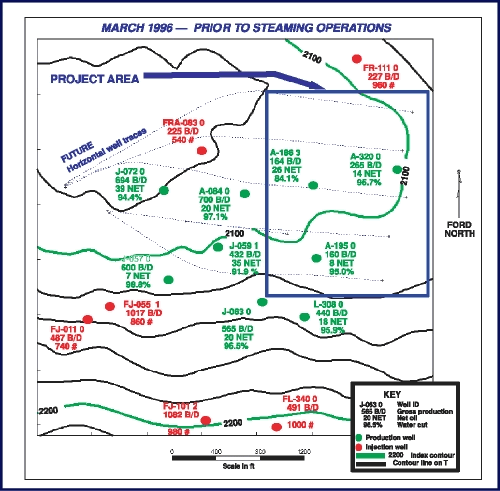
The five horizontal wells were steam cycled and placed on production (Figures 16, 17, and 18). Two of them, FJ- 204 and FJ-202, were placed on permanent steam injection. A-186 3, A-195 0, and A-320 0, each well more than 30 years old, remained on production within the steamproject boundaries. As of March 1996, they had averaged 2.5 m³/day (16 bbl/day) net with 31.8 m³/day (200 bbl/day) gross, at an average water cut of 92%.

When the horizontal project was initiated, this area had only about five years of remaining economic life under waterflood, and recoverable reserves were estimated at 11,924 m³ (75,000 bbl). The average pool-water cut prior to steaming was 95%. The water cut in the project area was 81% in 1998 and 92% in July 2000; another 270,283 m³ (1,700,000 bbl) of reserves has been added to the Tar V pool.

Steam communication to the existing waterflood wells, from cyclic steam injection into wells FJ-202 and FJ-204, resulted in a six- to tenfold net production increase in the old waterflood wells (Figure 17). Peak annual production rates under steam drive were forecast at 93.8 m³/day (590 bbl/day) for the horizontal project. During the first four months of 1998, the average oil production was 111 m³/day (698 bbl/ day). In July 2000, the average oil production was 38.5 m³/day (242 bbl/ day). The production rates should be several times greater, but the performance of each well has been hindered by fluid levels exceeding 457.2 m (1500 ft). The high fluid level suppresses oil production and cools the produced fluids, resulting in lower recoveries. The success of the program is reflected in Figures 16, 17, and 18, which show how the project area has changed over time. Note in Figure 16 that prior to steaming, the average net was about 2.5 m³ day (16 bbl/day). By January 1998 (Figure 17). the average net was more than 23.9 m³/day (150 bbl/day). In August 2000, the average net was still more than 15.9 m³/day (100 bbl/day).

Three-dimensional techniques contributed significantly to the success of the Tar zone horizontal project. Assuming a 50% recovery factor, every foot above the target is equivalent to 2524 STCM (15,876 STB) in lost reserves (Phillips, 1996). At U.S. $14/bbl oil, an error of as much as 1.5 m (5 ft) vertically would equate to U.S. $ 1.1 million in lost revenue.

Figure Captions (19-24)

	Figure 19. Three-dimensional display of the percentage of sandstone in the Hx₀ to Hx₂ interval of the Terminal zone in Fault Block V. Cartesian coordinate system is in feet, and vertical exaggeration is 2x.
	Figure 20. Three-dimensional display of qualitative oil saturation (So) for the Hx₀ sandstone of the Terminal zone in Fault Block V. Cartesian coordinate system is in feet, and vertical exaggeration is 2x. Oil saturation is posted with each well. Soc = current oil saturation; soi = initial oil saturation; So = oil saturation calculated from 1980s logs.
	Figure 21. Three-dimensional display of the Fault Block V Terminal zone showing the J-017 well and surrounding wells. The oil saturation is mapped within the Hx₀ sandstone. This is essentially a net-pay map for the Hx₀ sandstone.
	Figure 22. Three-dimensional bench-cut display showing the J-017 4 tight-radius sidetrack into the Hx₀ sandstones.
	Figure 23. Structure map of the Hx_0J sandstone showing the well course for J-017 4. The sandstone shales out and merges with the Hx_0J shale in the western portion of the area. Five-feet contour intervals are in feet vertical subsea. A small fault was detected during drilling and was incorporated into the model.
	Figure 24. J-017 4 horizontal-well log, showing logging-while-drilling (LWD) and modeled logs. An excellent match was obtained. The location of this well is shown in Figure 23.

Case History 3: Upper Terminal Zone: Hx₀ Thin-Sandstone Sequence

The Hx₀ sandstones of Fault Blocks V and VI were reviewed as part of a U.S. Department of Energy (DOE) class III short-term project (Phillips, 1998). The project proposed using new reservoir characterization tools and techniques to exploit bypassed oil. The new technologies included detailed reservoir characterization; 3-D geologic modeling; geosteering in thin, heterogeneous beds; and modeling the LWD responses (MacCallum et al., 1998).

A deterministic geologic model was created to define the Hx₀ layer and the horizons above and below it (Hx₁ above, Hx₂ and Hx below). The sandstone percentage was calculated for each data point. A 3-D property model was created by gridding the sandstone percentage in 3-D space using the top and bottom of the Hx₀ as confining surfaces (Figure 19). The original oil saturation (So) was property modeled similarly to identifying target areas for exploitation (Figure 20).

A display of the So model and wells drilled in the 1980s clearly showed that Fault Block VI was effectively drained, but Fault Block V still had reserves. The difference between the original So and that indicated by the 1980s wells was quantifiable. This is easily seen in Figure 20 for wells A-160 and A-189. The calculated So is less than 40%, whereas the property model shows the original So to be 60%. The So calculated from the old wells was decremented, the two data sets were combined, and Fault Block V was again property modeled (Figure 21). The sandstone percentage model and the So model were combined, and the original oil in place was calculated to be 540,566 STCM (3.4 million STB). The current oil in place was calculated, and the reserves were reduced to 445,172 STCM (2.8 million STB) (Phillips and Clarke, 1998). Obviously, significant reserves remain.

Based on the geologic model, the block engineer proposed that a horizontal well be drilled within and adjacent to the modeled area along the structural high. An existing wellbore was sidetracked with a horizontal lateral to capture hydrocarbon reserves not economically recoverable with conventional methods. Idle well J-017 was selected for drilling the high dogleg horizontal well, and a production rig was configured for drilling to keep costs to a minimum. By investigating the area west of the original Hx₀ project area, it was determined that the target sandstone thins and shales out to the west, thus reducing oil saturation. Electric logs from wells penetrating the area as far as 305 m (1000 ft) to the west were correlated, and a second 3-D geologic model was created.

A facies boundary was delineated to constrain the planned well course within the higher water-saturation (So) target. The Hx₀ layer was subdivided, and two sandstone lobes were identified within the Hx₀ layer. The Hx_0J and Hx_0B horizons were defined and added to the 3-D model. Maps and cross sections were extracted from the 3-D model and used for well planning (Figures 21 and 22).

A cross section along the well course was created for the geologist. The directional vendor required three linear cross sections for drilling because the well plan showed a U-turn (Figure 22). Stratigraphic sections consisting of adjacent wells also were created to help in geosteering. Both pasteup and digital varieties were used.

Structure maps were created on the Hx₁, Hx₀, and newly defined Hx_0J (Figure 23) and Hx_0B sandstones. These plots, as well as the 3-D model, were used for geosteering. Ultimately, they also were used for directional control because of rig-site problems.

A recently introduced, probe-based multiple-propagation- resistivity (MPR) device was used to provide LWD geosteering as well as directional information. This resistivity sensor was part of a slim-hole, positive-pulsetype MWD/LWD system that was used instead of carrier wave tools because of its smaller size (the tool diameter is 4 3/4 in.). These newer tools have well-integrated surface equipment, are battery-powered, and provide more reliable telemetry signals. The MPR tool is a four-transmitter, two-receiver array that provides a total of eight compensated resistivities at 2 MHz and the deeper-reading 400 kHz in boreholes as small as 5 7/8 in. For additional geosteering control, an inclinometer and gamma-ray scintillation detector are placed below the MPR sub (MacCallum et al., 1998). The well was successfully placed within two sandstone lobes of the thin sequence by geosteering using the LWD data.

The interval is thin and shaley (total thickness of 5.2 m [17 ft]), and the LWD showed the anisotropic effect throughout the log (Figure 24). The resistivity response in anisotropic conditions is similar to conductive invasion in that the short-spaced measurement reads less than the long-spaced for both the phase difference and attenuation resistivity measurements. However, the shallow-reading, phase-difference resistivity curves measure a higher resistivity than the deep-reading attenuation curves for both frequencies and spacings. This curve order is not indicative of conductive invasion but of anisotropy (Meyer et al., 1996). The presence of anisotropy plus formation heterogeneity complicated the interpretation of the LWD data so that the geosteering team had to rely significantly on the geologic model.

A simple layer model was used for previous horizontal-well projects. The sandstone package was thick enough that the LWD gave a unique, easily interpretable response. The Hx₀ sandstone is divided by a continuous shale. The upper sandstone, referred to as the Hx₀, is 1.8 m (6 ft) thick; the lower sandstone, Hx_0J, is 2.4 m (8 ft) thick. Again, the horizontal well was successfully placed into each of these sandstones.

Postwell analysis and support were excellent. The LWD analyst spent significant time studying the LWD data and explaining the results. For wells drilled parallel to bedding, adjacent beds and formation anisotropy were significant factors in the log response. The anisotropy was quantified, the horizontal and vertical resistivity was determined, and a mathematical model of the LWD response was created (MacCallum et al., 1998).

The 3-D model was refined based on conclusions reached by collaboration between the LWD analyst and the geologist. The shales above the Hx₀ and Hx_0J sandstones were modeled, which helped significantly in data interpretation. A new anisotropy inversion algorithm and the inclusion of shales in the geologic model allowed for a clearer understanding of the 2-MHz resistivity responses to the formation and their boundaries.

The fault geometry of a previously unidentified fault also was determined during this process using the 3-D model and further mathematical modeling of the LWD. There was a good correlation between the tops calculated from the 3-D geologic model and the tops selected from the LWD log. The average vertical distance between the bed boundary calculated from the 3-D geologic model and the well, as determined by the LWD log, is less than 0.08 m (0.25 ft).

Conclusions

A geologist working with carefully characterized rock data and 3-D modeling and visualization techniques adds greatly to a horizontal drilling team. The highly accurate 3-D visualizations of the reservoir greatly increase the confidence factor of the team, thus enabling Wilmington field reserves to be maximized.

To be effective, horizontal wells require precision placement. Three-dimensional models help isolate data inconsistencies, and 3-D viewers are good for adding data to correct the geologic model. Once the final geologic model is created, the drilling team can use the resulting 3-D visuals with confidence to improve drilling techniques and directional control. Postwell analysis of the LWD data also is facilitated using 3-D geologic models.

Acknowledgments

We would like to acknowledge the help and support of Mike Domanski, president of Tidelands Oil Production Company; Jim Quay, Steve Siegwein, Scott Walker, Scott Hara, Rudy “Bud” Payan, and Chris Parmelee, technical engineering staff at Tidelands Oil Production Company; Dennis Sullivan, director of the Department of Oil Properties, city of Long Beach; Donald McCallum of Baker-Hughes INTEQ; and Art and Tamara Paradis and Heather Kelley of Dynamic Graphics Inc. Computer modeling was done with DGI EarthVision on an SGI Iris Indigo workstation.

References Cited

Ames, L. C., 1987, Long Beach oil operation—A history, in D. D. Clarke and C. P. Henderson, eds., Geologic field guide to the Long Beach area: Pacific Section AAPG, p. 31–36.

Biddle, K. T., 1991, The Los Angeles basin: An overview, in K. T. Biddle, ed., Active margin basins: AAPG Memoir 52, p. 5–24.

Blake, G. H., 1991, Review of the Neogene biostratigraphy and stratigraphy of the Los Angeles Basin and implications for basin evolution, in K. T. Biddle, ed., Active margin basins: AAPG Memoir 52, p. 135–184.

Blesener, J. A., and C. P. Henderson, 1996, New technologies in the Long Beach Unit, in D. D. Clarke, G. E. Otott Jr., and C. C. Phillips, eds., Old oil fields and new life: A visit to the giants of the Los Angeles Basin: Pacific Section AAPG, p. 45–50.

California Department of Conservation, Division of Oil, Gas, and Geothermal Resources, 1999, 1998 annual report of the state oil and gas supervisor: California Department of Conservation, Sacramento, 269 p.

Clarke, D. D., 1987, The structure of the Wilmington oil field, in D. D. Clarke and C. P. Henderson, eds., Geologic field guide to the Long Beach area: Pacific Section AAPG, p. 43–56.

Davies, D. K., and R. K. Vessell, 1997, Improved prediction of permeability and reservoir quality through integrated analysis of pore geometry and openhole logs: Tar zone, Wilmington field, California: Society of Petroleum Engineers, SPE Paper 38262, 9 p.

Davies, D. K., R. K. Vessell, and J. B. Auman, 1997, Improved prediction of reservoir behavior through integration of quantitative geological and petrophysical data: Society of Petroleum Engineers, SPE Paper 38914, 16 p.

Henderson, C. P., 1987, The stratigraphy of the Wilmington oil field, in D. D. Clarke and C. P. Henderson, eds., Geologic field guide to the Long Beach area: Pacific Section AAPG, p. 57–68.

Koerner, R. K., D. D. Clarke, S. Walker, C. C. Phillips, J. Nguyen, D. Moos, and K. Tagbor, 1997, Increasing waterflood reserves in the Wilmington oil field through improved reservoir characterization and reservoir management: Annual report submitted to the U.S. Department of Energy, Cooperative Agreement Number DE-FC22- 95BC14934, unpaginated.

MacCallum, D., M. Pactel, and C. C. Phillips, 1998, Determination and application of formation anisotropy using multiple frequency, multiple spacing propagation resistivity tool from a horizontal well, onshore California: Society of Professional Well Log Analysts 39th Annual Logging Symposium, Keystone, Colorado, May 1998.

Mayuga, M. N., 1970, Geology and development of California’s giant Wilmington oil field, in Geology of giant petroleum fields—Symposium: AAPG Memoir 14, p. 158–184.

Meyer, W. H., T. Maher, and P. J. McLean, 1996, New methods improve interpretation of propagation resistivity data: Presented at the Society of Professional Well Log Analysts 37th Annual Symposium, Taos, New Mexico.

Otott, Jr., G. E., 1996, History of advanced recovery technologies in the Wilmington field, in D. D. Clarke, G. E. Otott, Jr., and C. C. Phillips, eds., Old oil fields and new life: A visit to the giants of the Los Angeles Basin: Pacific Section AAPG, p. 37–44.

Otott, Jr., G. E., and D. D. Clarke, 1996, History of the Wilmington field: 1986–1996, in D. D. Clarke, G. E. Otott, Jr., and C. C. Phillips, eds., Old oil fields and new life: A visit to the giants of the Los Angeles Basin: Pacific Section AAPG, p. 17–22.

Otott, Jr., G. E., D. D. Clarke, and T. A. Buikema, 1996, Long Beach Unit 3-D survey, in D. D. Clarke, G. E. Otott, Jr., and C. C. Phillips, eds., Old oil fields and new life: A visit to the giants of the Los Angeles Basin: Pacific Section AAPG, p. 51–55.

Phillips, C. C., 1996, Enhanced thermal recovery and reservoir characterization, in D. D. Clarke, G. E. Otott, Jr., and C. C. Phillips, eds., Old oil fields and new life: A visit to the giants of the Los Angeles Basin: Pacific Section AAPG, p. 65–82.

Phillips, C. C., 1998, Geological review of Hx₀ Sands, in U.S. Department of Energy, Increasing waterflood reserves in the Wilmington oil field through improved reservoir characterization and reservoir management: 1997 Annual Report, Contract No. DE-FC22-95BC7 4934, Appendix 1, 12 p.

Phillips, C. C., and D. D. Clarke, 1998, 3D modeling/visualization guides horizontal well program in Wilmington field: Journal of Canadian Petroleum Technology, v. 37, no. 10, p. 7–15.

Phillips, C. C., D. D. Clarke, and L.Y. An, 1998, Give new life to aging fields: Oil and Gas Investor, v. 39, no. 9, p. 106–115.

Redin, T., 1991, Oil and gas production from submarine fans of the Los Angeles Basin, in K. T. Biddle, ed., Active margin basins: AAPG Memoir 52, p. 239–259.

Slatt, R. M., S. Phillips, J. M. Boak, and M. B. Lagoe, 1993, Scales of geologic heterogeneity of a deep water sand giant oil field, Long Beach Unit, Wilmington field, California, in E. G. Rhodes and T. F. Moslow, eds., Frontiers in sedimentary geology, marine clastic reservoirs, examples and analogs: New York, Springer-Verlag, p. 263–292.

U.S. Department of Energy, 1999, Increasing heavy oil reserves in the Wilmington oil field through advanced reservoir characterization and thermal production technologies, partners: The city of Long Beach, Tidelands Oil Production Company (Tidelands), University of Southern California, and David K. Davies and Associates: 1996 Annual Report, Contract No. DE-FC22-95BC1 493, 85 p.

Wright, T. L., 1991, Structural geology and tectonic evolution of the Los Angeles Basin, California, in K. T. Biddle, ed., Active margin basins: AAPG Memoir 52, p. 35–134.