![]() Click to view this article in PDF format.
Click to view this article in PDF format.
Applications of Pre-Stack Depth Migration*
By
Richard Postma1
Search and Discovery Article #40029 (2001)
1Interactive Earth Sciences, Inc., Denver, CO.
*Adapted for online presentation from article by same author, entitled "Pre-Stack Can Avoid Distortions," in Geophysical Corner, AAPG Explorer, September, 1997. Appreciation is expressed to the author and to M. Ray Thomasson, former Chairman of the AAPG Geophysical Integration Committee, and Larry Nation, AAPG Communications Director, for their support of this online version.
|
|
A problem that has always plagued geologists and interpreting geophysicists is the fact that seismic data resemble a cross-section of the earth, but are displayed in time rather than depth. To tie well control to seismic, well logs must be scaled to time, using check shot surveys or velocity functions derived from other means. The vertical exaggeration changes with depth (because velocity usually increases with depth), thus distorting the perspective and changing the apparent dip of fault planes, etc. These problems, however, are minor compared with the structural distortions that occur when velocity varies laterally as well as with depth. A solution to these problems exists in the development of pre-stack depth migration. Click here for sequence of Figures 1 and 2. Figure
2. A 2-D Click here for sequence of Figures 1 and 2.
Click here for sequence of Figures 4 and 5. Figure
5. Seismic line in South Texas, with Click here for sequence of Figures 4 and 5.
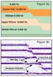
One of the principal motivators behind development of pre-stack depth migration was the desire to image seismic reflectors beneath salt structures. The abrupt velocity contrasts between the salt and adjacent sediment – coupled with the sometimes radical structural features associated with salt tectonics – produced severe distortions in the seismic travel times. The result is frequently a very poor stack and time pull-ups in the events that do stack. Time migration incorrectly migrates the distorted events because of the rapidly varying lateral velocities. An example of this from the Southern North Sea gas basin is shown in figures 1 and 2. Figure 1 is the 3-D time migrated line from a survey across two salt structures. The objective is the Rotliegendes sand beneath the Zechstein salt. The greatest velocity contrast is actually between the Cretaceous Chalk that has been forced upward by the salt movement, and the overlying Tertiary clastics. It is this Tertiary-Cretaceous boundary and the structure on it that produce the greatest distortion. Severe distortions can be seen in the Base Salt/Top Rotliegendes reflector beneath each of the structures. The event actually criss-crosses in a reverse “bow-tie” beneath the structure on the left. An apparent fault is seen beneath the structure on the right.
Another
more subtle example of the value of · They stack poorly. · The stacked traces have severe time distortion. Such
distortion can easily be interpreted as structure and/or secondary
faulting. Figures 4 and 5 show a comparison of a seismic line in South
Texas, with time migration and Other problem areas where depth migration can help include overthrust faults, channel fills, reefs, and karsted or eroded carbonate in the section above the zone of interest. In short, any time the objective lies beneath strata that have been disrupted by faulting, diapirism, etc. or show significant structural dip or where there are significant lateral variations in the overburden velocity, depth migration can be useful. There
are two reasons for performing depth migration · The velocity model can be derived directly from the data, usually with more accuracy than from stacking velocity or extrapolated well control. ·
The stack itself is disrupted and
degraded beneath velocity anomalies. Deriving and refining the velocity model is an iterative process, requiring numerous preliminary migrations and analysis cycles. Because of this, depth migration is expensive compared to other data processing procedures. However, it is cheap compared to the cost of drilling dry holes (see Figures 1 and 2)! |