![]() Click to view PDF version with images, as originally presented in AAPG
Explorer.
Click to view PDF version with images, as originally presented in AAPG
Explorer.
Stratton Field, South Texas: Example of Integration in Reservoir Characterization
By Bob A. Hardage
Search and Discovery Article #40020, (2001).
Senior research scientist, Bureau of Economic Geology at the University of Texas at Austin (www.beg.utexas.edu).
Adapted
for online presentation from two articles by same author, entitled
“Integration Aids Reservoir Effort” in Geophysical Corner, AAPG Explorer, December, 1997, and “Combining Data Aids
Interpretation” in Geophysical Corner, AAPG
Explorer, January, 1998. Appreciation is expressed to the author and to M.
Ray Thomasson, former Chairman of the AAPG Geophysical Integration Committee,
and Larry Nation, AAPG Communications Director, for their support of this online
version. For a somewhat expanded version of this B.E.G. study, the viewers are
referred to “3-D Seismic Imaging and Interpretation of Fluvially Deposited
Thin-Bed Reservoirs,” by Bob A. Hardage, R.A. Levey, V. ![]() Pendleton
Pendleton![]() , J. Simmons,
and R. Edson, in AAPG Studies in Geology No. 42, p. 27-33. This publication is
available from Bookstore at www.aapg.org.
, J. Simmons,
and R. Edson, in AAPG Studies in Geology No. 42, p. 27-33. This publication is
available from Bookstore at www.aapg.org.
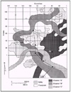
This article summaries a study of the Stratton Field, a large, Frio gas-producing property in Kleberg and Nueces counties in South Texas. The stratigraphic interval involved was the Oligocene Frio Formation – a thick, fluvially deposited sand-shale sequence that has been a prolific gas producer in Stratton Field and in several other fields along the FR-4 depositional trend (Figure 1). This reservoir-characterization effort is an example of integrating geophysics, geology, and reservoir engineering technologies to detect thin-bed compartmented reservoirs in a fluvially deposited reservoir system. An integrated interpretation of a complex reservoir system is made using 3-D seismic, well log, and bottom-hole pressure data. Techniques for thin-bed interpretations and recognition of reservoir heterogeneity are essential elements in the interpretation.
Two examples of seismic thin-bed interpretation in a fluvially deposited gas reservoirs are shown, and these interpretations are supported with geologic and reservoir engineering data. In these examples, the 3-D seismic data reveal stratigraphic variations where reservoir pressure information implies that a compartment boundary should exist. These examples illustrate that, although fluvial deposition creates numerous compartment boundaries, determining which seismically imaged stratigraphic changes are compartment boundaries requires that geologic and reservoir-engineering data (particularly reservoir-pressure data) be incorporated into the seismic interpretation.
In this study it was particularly important to have an accurate and reliable way to translate thin-bed stratigraphy (known in depth) into precisely defined seismic time windows. VSP data, when properly recorded and processed, are the best information to establish the detailed depth-versus-time calibration required to seismically distinguish closely spaced thin-beds. The VSP calibration procedure used was able seismically to distinguish thin-beds that are vertically separated by as little as 4 ms.
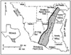 Figure
1--Index map showing FR-4 depositional trend in which Stratton Field is located.
Figure
1--Index map showing FR-4 depositional trend in which Stratton Field is located.
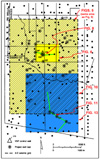 Figure
2--Map of Stratton field area, showing well locations and 3-D seismic grid.
Figure
2--Map of Stratton field area, showing well locations and 3-D seismic grid.
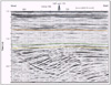
 Figure
3--Zero-offset image is spliced into a north-south vertical slice from the 3-D
data volume passing through the VSP well (Figure 2). Also shown is a graphic
representation of the stratigraphic column penetrated by the VSP well. The
F37 reservoir is about 20 feet above the F39 reservoir.
Figure
3--Zero-offset image is spliced into a north-south vertical slice from the 3-D
data volume passing through the VSP well (Figure 2). Also shown is a graphic
representation of the stratigraphic column penetrated by the VSP well. The
F37 reservoir is about 20 feet above the F39 reservoir.
 Figure
4--Continuous seismic reflection event imaged over the entire area by 3-D
seismic data, defining a geologic surface that corresponds to a fixed, constant
depositional time. Orange surface corresponds to C38 reservoir; green surface,
to F11 reservoir; and yellow surface, to F39 reservoir.
Figure
4--Continuous seismic reflection event imaged over the entire area by 3-D
seismic data, defining a geologic surface that corresponds to a fixed, constant
depositional time. Orange surface corresponds to C38 reservoir; green surface,
to F11 reservoir; and yellow surface, to F39 reservoir.
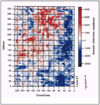
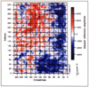 Figure
5--Reflection amplitude behavior on the F39 depositional surface shown in Figure
4.
Figure
5--Reflection amplitude behavior on the F39 depositional surface shown in Figure
4.
Click here for sequence of Figures 5 and 9 (for comparison of F37 and F39).
 Figure
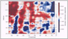
6--Magnified view of this F39 surface in the vicinity of four key wells.
Figure
6--Magnified view of this F39 surface in the vicinity of four key wells.
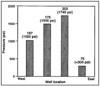 Figure
7--F39 reservoir pressure measurements that were acquired in all four wells. The
differences in these static pressures indicate that each well is in a different
F39 compartment.
Figure
7--F39 reservoir pressure measurements that were acquired in all four wells. The
differences in these static pressures indicate that each well is in a different
F39 compartment.
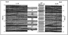
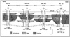 Figure
8--Stratigraphic correlation section that displays the available geologic
control. The log curves infer that the F39 reservoir in each well was deposited
in a channel environment with some evidence of splay deposition.
Figure
8--Stratigraphic correlation section that displays the available geologic
control. The log curves infer that the F39 reservoir in each well was deposited
in a channel environment with some evidence of splay deposition.
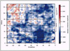
 Figure
9-- Reflection amplitude behavior on the F37 surface.
Figure
9-- Reflection amplitude behavior on the F37 surface.
Click here for sequence of Figures 5 and 9 (for comparison of F37 and F39).
 Figure
10--Enlargement of the meander features of F37.
Figure
10--Enlargement of the meander features of F37.
Click here for sequence of Figures 10 and 13 (seismic reflection event vs. model).
 Figure
11--Log-based stratigraphic cross-section of the F37 reservoir.
Figure
11--Log-based stratigraphic cross-section of the F37 reservoir.
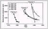 Figure
12--Rapid F37 pressure decay in well 189.
Figure
12--Rapid F37 pressure decay in well 189.
 Figure
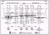
13--Multi-discipline reservoir model, illustrating the proposed model for F37
reservoir.
Figure
13--Multi-discipline reservoir model, illustrating the proposed model for F37
reservoir.
Click here for sequence of Figures 10 and 13 (seismic reflection event vs. model).
Thin-Bed Interpretation Procedure
Defining Chronostratigraphic Depositional Surfaces
The study covered a 7.6-square-mile area (Figure 2) where 3-D seismic data were acquired and where a large number of wells were used in making a geologic analyses of the Frio reservoirs. Additional well data (with well locations corresponding to the circled dots) were used to supplement the historic well log, production and reservoir pressure databases; they consist of modern well logs, cores, and various pressure tests.
Vertical seismic profile (VSP) data were recorded in two closely spaced wells inside the triangle shown near the center of the 3-D grid.
Thin-Bed Interpretation Procedure
The seismic interpretation at Stratton Field was particularly challenging because most of the Frio reservoirs are thin (<15 feet, or 5 meters), and they were closely stacked--in some areas individually separated vertically by only 10-15 feet (3-5 meters). These conditions required precise calibration of stratigraphic depth-versus-seismic travel-time to extract a depositional stratal surface from the 3-D data volume that would reliably depict the areal distribution of a particular Frio thin-bed reservoir. Zero-offset VSP data recorded in one of the wells shown in Figure 2 were used to establish the precise depth-versus-time control needed for the thin-bed interpretation. Figure 3 shows the zero-offset image spliced into a north-south vertical slice from the 3-D data volume passing through the VSP well. Also shown in Figure 3 is a graphic representation of the stratigraphic column penetrated by the VSP well. Only producing or potentially-producing Frio reservoirs are shown in this diagram, and not all of the reservoirs are labeled by name. The top and base of each reservoir are accurately positioned in terms of two-way VSP travel-time, and because there is no difference in the VSP and 3-D time datum in this case, the reservoirs are also correctly positioned vertically inside the 3-D seismic data volume at the VSP well.
Using these VSP travel-time control data, each thin-bed reservoir can be placed in the correct reflection phase position in the 3-D seismic reflection wavefield at the VSP well. This thin-bed calibration was extended away from the VSP well and across the entire 7.6-square-mile area imaged by the 3-D data using the interpretation principles of seismic stratigraphy.
Defining Chronostratigraphic Depositional Surfaces
The fundamental assumption made in the seismic interpretation was that seismic reflections follow chronostratigraphic depositional surfaces (Vail and Mitchum, 1977). Thus, a continuous seismic reflection even imaged over the entire 7.6-square-mile area by the 3-D seismic data defines a geologic surface that corresponds to a fixed, constant depositional time. Two such areally continuous reflection events were found in the Frio interval. These two surfaces are shown on the east-west vertical section crossing the VSP well (Figure 4).
At the VSP control well, the apex of the peak associated with the shallower stratal surface (the orange surface in Figure 4) corresponds to the thick C38 reservoir (Figure 3), and the apex of the peak at the deeper stratal surface (the green surface in Figure 4) correlates with the F11 reservoir. Thus, the seismic time surface following the apexes of all of the peaks of the orange event is assumed to define the ancient topographic Frio surface at the time when the C38 reservoir sediments were deposited.
Similarly the seismic time surface following the apexes of the peaks of the deeper green event define the ancient depositional surface associated with the F11 reservoir. Once the 3-D data volume was flattened relative to one of these two reference stratal surfaces, it follows that any horizontal time slice in this flattened data volume also followed an ancient Frio depositional surface – as long as the seismic reflection character in the immediate neighborhood of the time slice was time-conformable with the reflection character in the immediate vicinity of the reference surface used to flatten the data volume.
This interpretation is based on the assumption that the entire Frio section inside the 7.6-square-mile grid was seismically conformable to one of the two seismic reference surfaces. In this specific interpretation problem, with many closely spaced (vertically) thin-beds, the VSP-defined position of a particular thin-bed reservoir was rarely at the apex of a reflection peak or trough. Invariably, each thin-bed of interest was positioned at some intermediate, commonly non-descript phase point in the reflection waveform at the VSP control well.
To create a seismic image that emphasizes the internal complex architecture of a given thin-bed reservoir system, the migrated 3-D data volume was:
-
First time shifted so the proper pre-defined reference stratal surface was flat.
-
Then a horizontal time slice was made through this flattened data volume at the exact VSP-defined time for the targeted thin-bed, regardless of where that time slice is positioned in the reflection waveform at the VSP control well.
By prior assumption, the seismic time surface contained in this horizontal slice was the fixed depositional stratal surface where that thin-bed unit was deposited, and any seismic anomalies seen on this surface would be related directly to stratigraphic heterogeneities within the targeted thin-bed and, to a lesser degree, would be related to stratigraphic variations in thin-beds positioned immediately above and below the target thin-bed.
The F39 reservoir was the deepest Frio reservoir studied. (The depositional surface for the F39 reservoir is shown by the yellow horizon in Figure 4; the reflection amplitude behavior on the F39 depositional surface is shown in Figure 5.) The linear north-south trends near the center of the image are assumed to be residual effects from the deeper Vicksburg faults (a magnified view of this F39 surface in the vicinity of four key wells is shown in Figure 6).
F39 reservoir pressure measurements were acquired in all four wells (Figure 7), and the differences in these static pressures indicate that each well is in a different F39 compartment. The 3-D seismic image and the available geologic control gave clues as to where the boundaries are that segregate the F39 reservoir into these distinct compartments.
Figure 8 displays the available geologic control. The log curves infer that the F39 reservoir in each well was deposited in a channel environment that shows some evidence of splay deposition. The seismic image defines some possible compartment boundaries. For example, the most likely cause of the compartment boundary that separates well 197 from the other wells is the depositional variation that created the red/blue (positive/negative) amplitude changes, which trend north-south between crossline coordinates 130 and 140 (Figure 6).
Similarly, a probable seismic indication of the compartment boundary that segregates well 75 from the other wells is the positive-to-negative (red-to-blue) amplitude variations trending north-south between crossline coordinates 110 and 120. By analyzing the seismic, geologic, and engineering data associated with the F39 reservoir, it is possible to detect F39 reservoir compartments seismically--at least in the vicinity of wells 75, 175, and 197.
To create this reservoir compartment model, it is essential that the seismic image be interpreted with the assistance of reservoir-pressure data to infer which of the many stratigraphic changes revealed in the seismic image are most likely to be the compartment boundaries.
The F37 reservoir is approximately 20 feet (6 meters) above the F39 reservoir in the VSP calibration well (Figure 3). The two-way travel-time difference between F37 and F39 is only four milliseconds (4 ms). Using the thin-bed interpretation procedure above, a time slice was made through the flattened 3-D data volume 4ms above the F39 stratal surface. This F37 surface is displayed in Figure 9. Comparing this image with the F39 surface (Figure 5), red, linear north-south apparent channels in the central part of the F37 image are similar to those observed in the F39 image, implying that Vicksburg faulting was still controlling sedimentation in this part of the field.
However, there is a significant difference in the southeast quadrant of the F39 and F37 images. Specifically, meander channel features occur at the F37 level but are not present at the deeper F39 surface. (An enlarged plot of the meander features in Figure 9 is shown on Figure 10.) A log-based stratigraphic cross-section of the F37 reservoir across the meander features and extending southward beyond the seismic grid was constructed (Figure 11). The depositional environment (either channel or splay) at each well is an interpretation based on log-curve shape and was made before the 3-D seismic data were recorded.
This geologically-based interpretation of the F37 depositional environments indicates that the meander feature seen in the F37 seismic surface is indeed a depositional channel. Specifically, the log interpretation (Figure 11) implies the F37 reservoirs found in wells 189 and 185 were deposited as channel fill, and the seismic image shows these wells to be coincident with a meander feature.
The interpretation of depositional environment for the extremely thin F37 reservoir in well 211 is a splay (Figure 11). The 211 wellhead is approximately 300 feet (91 meters) north of the meander feature (Figure 10). The log-based interpretation of the F37 depositional environment at the 211 well is thus supported by seismic evidence.
Pressure histories recorded in several F37 reservoirs near these seismic meander features were analyzed to determine if reservoir compartmentalization exists. These pressure histories (Figure 12) show there are at least three, and perhaps four, individual F37 reservoir compartments in this area of the field.
A proposed reservoir model that honors all three databases--seismic, geologic, and reservoir engineering--is shown in Figure 13. This model assumes that the F37 reservoir in the southeast quadrant of the 3-D grid is composed of three intermeshed channels, labeled A, B and C, and a grid overlay of seismic inline and crossline coordinates is provided so these channels can be correlated with features in the 3-D seismic image.
The location of the F37 stratigraphic cross-section (Figure 11) is shown, but this geologic information defines channel locations along only a single 2-D profile of the model. The important information is the reservoir-pressure data, because without this engineering data there would be no reason to conclude that a three-channel model would be appropriate. Thus, the reservoir-compartment model places well 129 in Channel A and well 185 in Channel B; this allows these two wells to be in different F37 pressure regimes; i.e., in different compartments (channels).
Wells 127 and 161 are proposed to be in channel C, south of the 3-D seismic coverage. Only one meander loop of this hypothesized channel C extends into the 3-D seismic grid. The rapid F37 pressure decay observed in well 189 (Figure 12) implies that this well is not in pressure communication with well 185, even though both wells are in channel B. There may be an intrachannel compartment boundary in channel B.
The reservoir model in Figure 13 is hypothetical and may not yet be the correct picture of the compartmentalized nature of these F37 reservoirs. However, the F37 reservoir in this portion of Stratton Field is segregated into distinct compartments, and this compartmentalization must be caused by the variable elements of fluvial deposition, because the seismic data show no evidence of faulting in these particular reservoirs.
The proposed reservoir model honors all existing data that provide any information about the F37 reservoir system. The seismic image in Figure 10 reveals not just one meander channel system but at least three intermeshed thin-bed channels. By using pressure histories it was possible to use 3-D seismic images to define where compartment boundaries most likely exist in the interwell space.
Raymond
A. Levey, ![]() Virginia
Virginia![]()
![]() Pendleton
Pendleton![]() , James Simmons and Rick Edson, all at the Bureau of
Economic Geology at the time this work was done, assisted in the writing.
, James Simmons and Rick Edson, all at the Bureau of
Economic Geology at the time this work was done, assisted in the writing.