3-Dimensional
Digital Outcrop ![]() Data
Data![]() Collection and Analysis
Using Eye-safe Laser (LIDAR) Technology*
Collection and Analysis
Using Eye-safe Laser (LIDAR) Technology*
By
Jerome A. Bellian1, David C. Jennette1, Charles Kerans1, James Gibeaut1, John Andrews1, Brad Yssldyk2, David Larue3
Search and Discovery Article 40056 (2002)
*Adapted for online presentation from poster session at AAPG Convention, Houston, Texas, March 2002.
1The Bureau of Economic Geology, The University of Texas at Austin, TX ([email protected]; [email protected]; [email protected]) (www.beg.utexas.edu)
2Optech, Toronto, ON
3Chevron Petroleum Technology Company, San Ramon, CA ([email protected])
* Editorial Note: This article, which is highly graphic (or visual) in design, is presented as: (1) three posters, with (a) each represented in JPG by a small, low-resolution image map of the original; each illustration or section of text on each poster is accessible for viewing at screen scale (higher resolution) by locating the cursor over the part of interest before clicking; and (b) each represented by a PDF image, which contains the usual enlargement capabilities; and (2) searchable HTML text with figure captions linked to corresponding illustrations with descriptions.
Users without high-speed internet access to this article may experience significant delay in downloading some illustrations due to their sizes.
First Poster
Second Poster
Third Poster
Fourth Poster
Fifth Poster
Abstract
New efforts to integrate critical ground truthing from outcrop ![]() data
data![]() into the
rapidly evolving world of digital subsurface mapping and exploration have taken
significant strides in the last decade. LIDAR (Light Detection And Ranging), a
laser-based mapping tool developed for atmospheric studies in the mid-1960s,
enables geologists to rapidly and accurately collect stratigraphic information
directly from outcrops scanned with intensity-sensitive laser instrumentation.
Light-ranging
into the
rapidly evolving world of digital subsurface mapping and exploration have taken
significant strides in the last decade. LIDAR (Light Detection And Ranging), a
laser-based mapping tool developed for atmospheric studies in the mid-1960s,
enables geologists to rapidly and accurately collect stratigraphic information
directly from outcrops scanned with intensity-sensitive laser instrumentation.
Light-ranging ![]() data
data![]() is co-rendered with laser intensity
is co-rendered with laser intensity ![]() data
data![]() to generate 3D
outcrop models with near zero distortion in x, y and z space. In addition, the
intensity of the return signal helps to discriminate between different
lithologic types. The results can be likened to black and white photography
draped onto a 3D surface.
to generate 3D
outcrop models with near zero distortion in x, y and z space. In addition, the
intensity of the return signal helps to discriminate between different
lithologic types. The results can be likened to black and white photography
draped onto a 3D surface. ![]() Data
Data![]() acquisition can be done in any lighting
conditions, with a rate of 2000 points per second.
acquisition can be done in any lighting
conditions, with a rate of 2000 points per second.
This instrument
can achieve sub-centimeter range resolution with 16-bit intensity returns for
each ranging point recorded. A 1 x 0.3 km outcrop face can be acquired and
merged into a single point-cloud dataset with corresponding intensity in less
than two hours on a standard laptop computer. Case studies include deepwater
carbonate and siliciclastic outcrops from West Texas and deepwater channel
sandstones from northern Spain. These ![]() data
data![]() are ideal for display and
interpretation on workstation systems. Results are then directly imported into
subsurface
are ideal for display and
interpretation on workstation systems. Results are then directly imported into
subsurface ![]() modeling
modeling![]() software to measure and collect fine-scale bed-length
software to measure and collect fine-scale bed-length ![]() data
data![]() and to construct remarkably accurate architecture and lithofacies models.
and to construct remarkably accurate architecture and lithofacies models.
|
|
Figure Captions (Concept, Workflow, and Model; Figures 1-1 to 1-7)
3D Outcrop to 3D Model Concept and Workflow
· Interpretation: Add stratigraphic interpretation to 3D photo-draped outcrop model.
The
workflow for generating a photo-draped 3D outcrop model used as a
foundation for complex geological models (Figure
1-1) begins with point
cloud
LIDAR at The University of Texas at Austin
This thing called “LIDAR” is an acronym that describes a method of determining position of a target relative to some arbitrary reference point (Figure 1-2). LIDAR stands for Light Detection and Ranging. It was originally used by atmospheric and planetary geoscientists in the 1960s to image bodies of galactic matter and atmospheric plumes. LIDAR is Light Detection and Ranging; RADAR is Radio Detection and Ranging; SONAR is Sound Navigation and Ranging. LIDAR can be compared to other remote sensing techniques such as SONAR and RADAR, which also determine the position of distant targets from a known point.
The University of Texas at Austin is the only University in the world with Optech ALTM airborne and ILRIS 3D ground-based LIDAR instruments (Figures 1-3, 1-4, 1-5). The combination of these two instruments enables us to survey entire cities at up to millimeter point spacing in 3D.
Points and Intensity to Surface Model (Figure 1-6)
Point clouds are “smart-filtered” to eliminate
excessive
A full-resolution intensity image is then
matched to the terrain model. Since the intensity is from the x, y, and
z laser return, it matches exactly to the TIN (3.),
Figure 1-6). The
result is a pseudo-black and white 3D photograph derived from
laser-returned x, y, z and intensity
Digital Terrain Model-Photo Merge (Figure 1-7)
The process of adding a photograph to the x, y, z, and intensity model uses a “rubber-sheet” rectification technique (we used ER Mapper for this), where multiple control points are picked on each photo that correspond to points on an intensity image (Figure 1-7). Between 30 and 60 control points are used depending on the terrain complexity. Picking control points is fast and easy since the photo and the intensity image are acquired at the same time from the same vantage point. To generate a true 3D effect, we use angular variance normal to the dataset origin to define a best-fit image to color-map to the x, y, z pixels. For example, if the user wants to display all faces > 90 degrees from the normal to the TIN face with color pixels from image 1 and all faces from < 90 degrees with color pixels from image 2, this can be done using a “normal gate” as follows:
If (q>90) then C = Image1; if q<90 then C = Image2 Where q = viewers perspective angle with reference to face normal and C = color pixels to be mapped.
The technique allows us to map multiple images onto a single surface resulting in a full 3D textured surface. The textured surface is now optimized to any viewer perspective allowing the viewer to “see” around corners with full resolution. This technique also reduces “doubling up” of images from multiple perspectives and thereby reduces rendering time.
Figure Captions (Deep-Water Clastic Case Studies; Figures 2-1 to 3-8)
Deep-Water Clastic Case Studies
Ainsa, Northern Spain (Photo Drape)
The map view of the Ainsa 2 outcrop (Figure
2-1) shows the general outcrop trend were
The Ainsa deep-water sandstone outcrop from
Northern Spain was selected to demonstrate the minimum level of
resolution currently being achieved at the Jackson School of Geosciences
at the University of Texas at Austin. The green pixels in the intensity
images (Figure 2-3) are keyed to a linear cutoff of intensity values
coded to display as green. Combining the image RGB and Intensity image
improves the ability for us to remove vegetation without loosing
valuable geological details. It also opens up the potential to use gated
logic statements to filter out unwanted
Intensity TIF + Original photo = Photo mapped onto intensity TIF Photo mapped onto intensity TIF
Photo mapped onto intensity TIF + X, Y, Z TIN = 3D photo draped model 3D photo draped model
Ainsa Quarry, Northern Spain (Variable Perspective)
The two images in Figure 2-5 illustrate
perspective correction possibilities when using LIDAR. The photo mosaic
(Figure 2-6) was taken from the same perspective as the ILRIS 3D
Brushy Canyon Formation, West Texas (Sand-Shale Discrimination)
Point clouds are assembled directly from
individual x, y, z, and intensity
The scans in Figures
3-1, 3-2, 3-3,
3-4 are
displayed in order to demonstrate that ILRIS 3D operates nearly
identically to a conventional camera in so much as ILRIS 3D acquires
image
Solitary Channel, Southern Spain (3-Dimensionality Across Multiple Fault Blocks)
In Figure 3-5, each color indicates an individual dataset used to reconstruct the Solitary Channel, outcrop. For comparison, the same image displayed also in Figure 3-5 with intensity of each x, y, and z point in grayscale.
Figure 3-6 displays this tractional,
conglomeratic channel fill by means of a photograph, an ILRIS 3D
intensity image, and the same intensity image draped onto the TIN
digital terrain model. The model enables the user to extract real
dimensional
The Solitary Channel Outcrop in Southern Spain
(Figures 3-5, 3-6,
3-7, 3-8) is an excellent
mixed-conglomeratic/sandstone outcrop analogous to many clastic, West
African, deep-water reservoirs. Understanding reservoir geometry and
continuity at the sub-
Figure Captions (Carbonate Case Studies; Figures 4-1 to 4-6)
Carbonate Case Studies:Upper Hueco - Clear Fork Formations, West Texas: (Basin Geometry)
Shown on a digital elevation model of the Sierra Diablo Mountains (Figure 4-1) is the mouth of Victorio Canyon, where good outcrops of the Upper Hueco through Clear Fork Formations on both north- and south-facing canyon walls. The focus for this study is the area of north facing wall (blue box in Figure 4-2). It was scanned using Optech Laser Imaging’s ILRIS 3D ground-based LIDAR instrument in February, 2002 (Figure 4-3). The cross-section in Figure 4-4 illustrates slope and toe of slope deposits (late Wolfcampian through early Leonardian) Victorio Canyon, West Texas, that crop out along the north-facing wall of Victorio Canyon.
The images in Figure 4-5 illustrate both the
photo pan and the ILRIS 3D LIDAR scan of the north facing wall of
Victorio Canyon. The photo pan has stratigraphic interpretation in red,
white and yellow whereas the ILIRS 3D point cloud does not. The transfer
of these
The images in yellow and green boxes in Figure
4-6 are moderate resolution TIN and intensity images generated from the
ILRIS point cloud Return to top.
Figure Captions (Long-Range Goals, Looking
Long-Range Research Goals at the Bureau of Economic Geology
Ground based LIDAR (Figure
5-2) is a tool that
provides geologists a quick, accurate, quantitative tool to better
understand stratigraphic relationships at the sub-
Conclusions
Photo-pan geology has worked well for us in
the past, much in the way that 2D
Looking
|
 Figure 1-5. Ground-based LIDAR instrument.
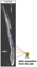 Figure 2-1. Map view of Ainsa 2 outcrop,
showing the general outcrop trend.
Figure 2-1. Map view of Ainsa 2 outcrop,
showing the general outcrop trend.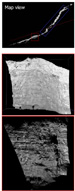 Figure 2-5. The two images illustrate
perspective correction possibilities with use of LIDAR, along with index
map of Ainsa quarry.
Figure 2-5. The two images illustrate
perspective correction possibilities with use of LIDAR, along with index
map of Ainsa quarry. Figure 2-6. Photo mosaic (upper) taken from
the same perspective in Ainsa quarry as the ILRIS 3D
Figure 2-6. Photo mosaic (upper) taken from
the same perspective in Ainsa quarry as the ILRIS 3D  Figure 2-7. Images of the same outcrop as that
in
Figure 2-7. Images of the same outcrop as that
in Figure 3-2. Another view of the stratigraphic
section in Guadalupe Canyon containing the channel complex--to
illustrate that ILRIS 3D acquires image
Figure 3-2. Another view of the stratigraphic
section in Guadalupe Canyon containing the channel complex--to
illustrate that ILRIS 3D acquires image  Figure 3-4. Blown-up image of the “100-foot
Channel” point-cloud dataset, along with close-up view of individual x,
y, z, and intensity points displayed with a grayscale color bar.
Figure 3-4. Blown-up image of the “100-foot
Channel” point-cloud dataset, along with close-up view of individual x,
y, z, and intensity points displayed with a grayscale color bar. Figure 3-6. Conglomeratic channel fill,
Solitary Channel, Southern Spain. Photo (upper left); ILRIS 3D intensity
image (upper right); Same intensity image draped onto the TIN digital
terrain model (lower right).
Figure 3-6. Conglomeratic channel fill,
Solitary Channel, Southern Spain. Photo (upper left); ILRIS 3D intensity
image (upper right); Same intensity image draped onto the TIN digital
terrain model (lower right). Figure 3-7. Solitary Channel outcrop, Southern
Spain: photograph, images, and block diagram.
Figure 3-7. Solitary Channel outcrop, Southern
Spain: photograph, images, and block diagram. Figure 4-2.
Victorio Canyon, with outline of the area of the north-facing canyon
wall that was scanned.
Figure 4-2.
Victorio Canyon, with outline of the area of the north-facing canyon
wall that was scanned. Figure 4-3.
Photograph of the north-facing canyon wall, Victorio Canyon, where
Figure 4-3.
Photograph of the north-facing canyon wall, Victorio Canyon, where  Figure 5-2. Photograph of the operation of a
ground-based LIDAR instrument.
Figure 5-2. Photograph of the operation of a
ground-based LIDAR instrument. Figure 5-5. A larger scale window of the
intersection in the foreground of the image in
Figure 5-5. A larger scale window of the
intersection in the foreground of the image in