The Linkage of Subsurface Natural Fracture Predictions With Oil Generation Estimates

M. K. Horn

Search and Discovery Article #40003 (1999)

*Adapted from a study in Basin History CD, which currently contains 640 worksheet based studies offered by AAPG Data Systems.

ABSTRACT
INTRODUCTION
THE STRESS HISTORY MODEL
THE HYDROCARBON GENERATION MODEL
LINKING THE HYDROCARBON GENERATION MODEL WITH THE OIL GENERATION MODEL: COMPUTATION OF FRACTURE OIL INDEX (FOI)
THE UINTA BASIN AND ALTAMONT BLUEBELL FIELD
ALTAMONT BLUEBELL RESULTS
COMPARISON OF UINTA RESULTS WITH A GLOBAL SAMPLE
CONCLUSIONS
FIGURES
APPENDIX I
APPENDIX II
REFERENCES

ABSTRACT

The Uinta basin of Utah contains oil and gas in fractured reservoirs. The Altamont-Bluebell field of this basin is chosen in order to test a concept that could be used to predict hydrocarbon-rich fractured reservoirs in, not only other parts of the Uinta, but in basins in other parts of the world.

The premise of the concept is to quantitatively predict the simultaneous occurrence of fracture formation and hydrocarbon generation. The advantage of such a prediction is that early emplacement of hydrocarbons in fractures enhances the probability of the said fractures remaining open through time; therefore enhancing reservoir potential. The early emplacement of hydrocarbons in fractures inhibits post-fracture diagenetic healing. Also, fluid pressures associated with the hydrocarbons would assist in maintaining fracture permeability.

Two well-established models are used to a) predict fracture formation as a function of burial history; and b) predict hydrocarbon generation also as a function of burial history. The two models are combined to produce a unique indicator, called the Fracture Oil Index or FOI. An FOI of less than -1 is an indicator of hydrocarbon-rich fractures. Using EXCEL spreadsheet formats, the calculated minimum FOI for the Eocene Green River Formation in the Altamont-Bluebell field is -58, which occurred 13 Ma at a burial depth of 5.73 km (18,800 ft). The -58 FOI ranks 62 out of 640 in technique-related global studies carried out in 174 basins (60 studies yielded FOI’s less than -58).

INTRODUCTION

Natural fractures provide important reservoir targets (Nelson, 1985, Appendix I; Fritz et al, 1985; Chilingar et al, 1972; Hubbert and Willis, 1955; Daniel, 1944). From an oil and gas exploration standpoint, fracture permeability is a prime requisite: the loss of fracture permeability greatly reduces reservoir potential. Permeability can be greatly reduced by diagenetic material filling the width between the walls of fractures (Nelson, 1985, p. 30).

One possibility for keeping fractures open is the injection of hydrocarbons into the fracture space(s) at the time, or immediately after, the formation of the fractures. Hydrocarbons in pore and fracture spaces are known to inhibit post-depositional diagenetic effects such as quartz overgrowth formation.

The challenge, then, becomes the prediction of the hydrocarbon generation occurring more or less simultaneously, through geologic time and at a specific locality, with natural fracture formation.

What we propose is to use the methods of Hunt et al (1991) to predict oil and gas generation potential and to link this with the Narr and Currie’s (1982) stress analysis predictor model. The resulting technique, utilizing EXCEL spreadsheet solutions, breaks down into the following steps for a specific locality:

1. Digitize and display the burial history of the target site.

2. If more than one burial history is provided at the target site, choose one candidate most probably linked to hydrocarbon source.

3. At the 1 km depth on the burial history curve, determine the corresponding geologic age. From the latter value (given as negative Ma for use in calculations), divide the total time to the present into 15 time segments. Read off the burial history curve the corresponding 15 paleo-depths.

4. From the paleo-depths, compute the paleo-temperature at each of the 15 stations. Use the present-day geothermal gradient for this computation if the paleo-temperature from other sources are not available.

5. Using the paleo-temperatures derived from 4 above, compute oil/gas generation curves for four activation energies, IIa Fast, IIB Medium Fast, IIC Medium, IID Slow (Hunt et al, 1991) at each of the fifteen stations. Also compute oil/gas generation curves at each of the fifteen stations using the Lopatin (1971) method.

6. At the exact same paleo-time stations, and again using the paleo-temperatures derived from 3 above, compute paleo-stresses using the Narr and Currie (1982) model.

7. In order to link the stress with hydrocarbon generation, at each of the paleo-time stations, multiply the oil generation percent by the minimum horizontal effective stress. Use the "correct" activation energy (see 5 above), or the Lopatin solution, when activation energies are not available. The resulting (arbitrary and relative) index, called FOI, will be negative and large when the potential for oil/gas generation occurs more or less simultaneously with natural fracture formation.

The above steps will be carried in the Altamont-Bluebell field area of the Uinta basin, Utah (Figure 1). Before we present these results, let’s review the stress history and oil generation models used in this study.

THE STRESS HISTORY MODEL

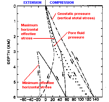
As rocks are buried, overburden weight causes stresses within the rock. Vertical stress can be "translated" into horizontal stresses, which may, in fact become extensional in nature. Extension leads to vertical fracture formation. Among the factors that cause variations in the state of stress within a rock are temperature changes, pore pressure, tectonic loading; and certain rock properties such as Young’s Modulus (rock rigidity) and Poisson’s ratio (used to relate horizontal stress components to vertical stress component) . These multitude of factors have been investigated and quantified by Narr and Curry (1982). Appendix I reviews the Narr and Curry stress history model in terms of stress prediction and related equations, and Figure 2 graphically displays some of their results. We are particularly interested in the minimum horizontal effective stress, s_y.

Of interest in the Narr and Curry model is the non-reversabilty of certain processes as a rock goes through its burial - diagenesis - uplift cycle. For example, as rocks are uplifted from their deepest point of burial to shallower depths, rock rigidity cannot become "undone" - the maximum value of Young’s Modulus is imprinted and remains as such as uplift proceeds. These irreversible processes affect the stress burial history.

We have taken the equations of Appendix I and rewritten them in spreadsheet (EXCEL) format. They are then used as described in Step 6 of the introduction.

THE HYDROCARBON GENERATION MODEL

The hydrocarbon generation model used in this study is that reported by Hunt et al in 1991. In this model, the time and depth of oil generation from petroleum source rocks containing type II kerogens are determined using time-temperature index (TTI) calculations based on the Arrhenius equation. Activation energies (E) and frequency factors (A) used in the Arrhenius equation were obtained from hydrous pyrolysis experiments.

Activation energies of standard kerogens vary inversely with their sulfur content (Hunt et al, 1991). The kerogen with the highest sulfur content has the lowest E value and is the fastest in generating oil, whereas the kerogen with the lowest sulfur content has the highest E value and is the slowest in generating oil. Hunt et al (1991) designated kerogens as types IIA, B, C, and D on the basis of decreasing sulfur content and corresponding increasing time-temperature requirements for generating oil.

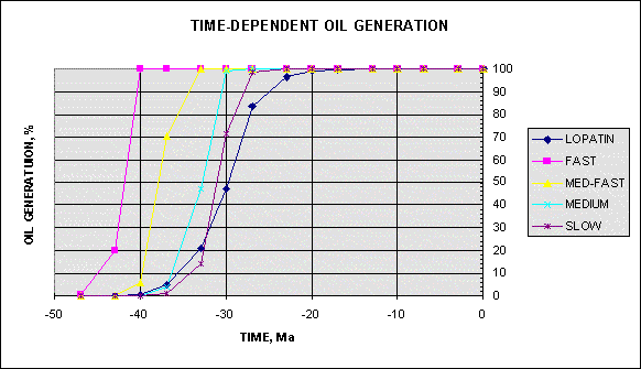
In our scheme, we use the E and A values in order to compute and construct EXCEL worksheet graphs that define oil generation as a function of geologic time. The results are reported within the range zero to 100 percent. Computed values greater that 100 percent are assumed to be in the thermal gas generation range. We display five oil generation curves (on one plot); Four of the five curves represent types IIA, B, C, and D; the fifth curve represents the Lopatin (1971) solution. We use Hunt et al’s (1991) equations 3 and 4 (shown as equations 2 and 3 in Appendix II of this study). Figure 3 is an example display of our oil generation EXCEL solution.

The constants used in order to solve the equations of Appendix II are:

">(FREQUENCY FACTOR, 1/m.y.)

	IIA	IIB	IIC	IID
	FAST	M. FAST	MEDIUM	SLOW
S (ORG), %:	1.1E+01	9.0E+00	7.4E+00	5.4E+00		(ORGANIC SULFUR)
E:	1.4E+02	1.8E+02	2.0E+02	2.2E+02		(ACTIVATION ENERGY, kJ/mol)1
A:	7.0E+20	4.2E+23	1.5E+25	5.7E+26		(FREQUENCY FACTOR, 1/m.y.)
R:	8.3E-03
R:	8.3E-03	8.3E-03	8.3E-03	8.3E-03		(GAS CONSTANT)

^1. Divide by 4.184 to convert to Kcal/mol

Although type II kerogens are the major oil generators in the world and were used to construct the hydrocarbon generation model, we also use, in lieu of more sophisticated data, the model for Type I kerogens. This, as will be seen, pertains to the Uinta basin.

LINKING THE HYDROCARBON GENERATION MODEL WITH THE OIL GENERATION MODEL: COMPUTATION OF FRACTURE OIL INDEX (FOI)

Fracture Oil Index (FOI) is defined as the product of minimum horizontal effective stress s_y and oil generation percent (Horn, 1995). An FOI of less than -1.0 is an indicator of hydrocarbon fracture potential. In our EXCEL solution, the calculation is made 15 times, at each of the previously described time stations on the burial history curve.

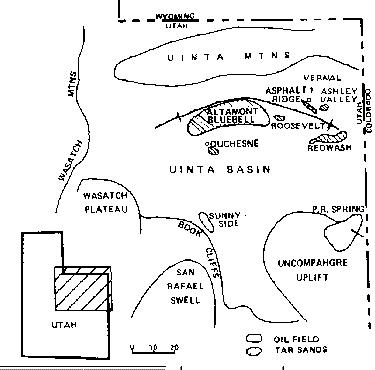
THE UINTA BASIN AND ALTAMONT-BLUEBELL FIELD

Typical of foredeep basins world-wide, the Uinta basin of Utah (Figure 1) is asymmetrical, with the basin depocenter lying close to the northern buttressed end of the basin. Depths reach 20,000 ft (6095 m) in the basin depocenter.

Uinta basin was created by the indentation of the Colorado Plateau into the North American craton during the Laramide plate movements (Harthill and Bates, 1996). Postdepositional shift of the structural axis of the basin in late Tertiary time produced a regional updip pinchout of northerly derived sandstones into a lacustrine "oil-shale" sequence (Lucas and Drexler, 1976). Fracture directions are N15°-50°W. At the Altamont-Bluebell field,VSP surveys defined N35°W as the open fracture direction (Harthill and Bates, 1996).

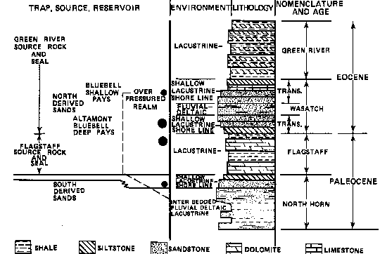
In the Uinta basin, the term oil shale refers to fine-grained rock that contains a large amount of organic material. (Sweeney et al, 1987). Strata of the Green River Formation were formed in a lacustrine environment that began in the middle to late Paleocene and reached maximum extent in middle Eocene time. Varves that can be traced over kilometers contain organic and inorganic matter deposited in yearly cycles. The organic material is mostly amorphous kerogen derived from the lipid fraction of lake algae and from terrestrial spores and pollen (Yen, 1976). This kerogen is a classic example of a Type I kerogen in the classification scheme of Tissot and Welte (1978).

Altamont Bluebell reservoirs occur on the gently dipping southern limb of the Uinta basin. Production occurs in the Eocene Green River - Wasatch section and Paleocene Flagstaff Limestone between depths of 7,875 and 16,735 ft (2,400 and 5,100 m). The producing interval is up to 2,300 ft (700 m) thick. Reservoir rocks are predominantly low-porosity, fine-grained sandstone, siltstone, and carbonate. The reservoir is substantially overpressured; the ratio of fluid pressure to overburden weight locally exceeds values of 0.8, and values in excess of 0.6 occur over an area greater than 772 mi² (2,000 km²) (Lucas and Drexler, 1976, Narr and Currie 1982). Structural closure plays no part in entrapment of hydrocarbons at Altamont-Bluebell; regional dip provides the setting for updip porosity pinchouts. Fractures in the reservoirs of essential for commercial flow rates. The reservoirs are essentially self-sourcing (Figure 4) with migration paths dependent upon fracture clusters. Initial well productivities were at flow rates up to 5,000 bbl/day with gas/oil ratios ranging from 1,500 cu ft/bbl (4,250 m³/bbl) in the updip part of the field to 500 cu ft/bbl (1,415 m³/bbl) downdip. Reservoir drive mechanism is liquid expansion-solution gas (Lucas and Drexler, 1964). In 1955 Carter No. 2 Bluebell Unit discovered gas (5.37 million cu ft/day) in sandstone in the Green River Formation (Osmond et al, 1968).

ALTAMONT-BLUEBELL RESULTS

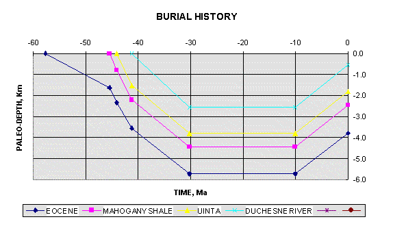
We shall now repeat the seven steps presented in the introduction, applied directly to the Shell 1-11B4 Brotherson well, Altamont-Bluebell field, Utah.

1. Digitize and display the burial history of the target site.

Figure 5 represents the EXCEL-graphed burial history, derived from a scanned image of Figure 11 of Sweeney et al (1987). The burial history represents the Shell 1-11B4 Brotherson well.

2. If more than one burial history is provided at the target site, choose the candidate most probably linked to hydrocarbon source.

The Eocene burial history curve is chosen.

3. At the 1 km depth on the burial history curve for the candidate source, determine the corresponding geologic age. From the latter value, divide the total time to the present into 15 time segments. Read from the burial history curve the corresponding paleo-depths. Note that for purposes of calculation, time values are given in -Ma.

TIME	TIME	DEPTH	DEPTH
START	FINISH	START	FINISH
Ma	Ma	Km	Km
-50.0	-47.0	-1.01	-1.45
-47.0	-43.0	-1.45	-2.64
-43.0	-40.0	-2.64	-3.83
-40.0	-37.0	-3.83	-4.48
-37.0	-33.0	-4.48	-5.11
-33.0	-30.0	-5.11	-5.70
-30.0	-27.0	-5.70	-5.73
-27.0	-23.0	-5.73	-5.73
-23.0	-20.0	-5.73	-5.73
-20.0	-17.0	-5.73	-5.73
-17.0	-13.0	-5.73	-5.73
-13.0	-10.0	-5.73	-5.68
-10.0	-7.0	-5.68	-5.13
-7.0	-3.0	-5.13	-4.40
-3.0	0.0	-4.40	-3.83

4. From the paleo-depths, compute the paleo-temperature at each of the 15 stations. Detailed analysis of temperature data by Chapman et al (1984) provides an estimate of 25°C/km for the present-day geothermal gradient in the Uinta basin. Sweeney et al (1987) assumed that the geothermal gradient from the Tertiary to the present has been constant, and they ignored localized effects on thermal gradient by factors such as overpressuring, lithologic variation, and hydrothermal circulation. A value of 10°C is chosen for the long-term average surface temperature.

TIME	TIME	DEPTH	DEPTH	TEMP	TEMP.
START	FINISH	START	FINISH	START	FINISH
Ma	Ma	Km	Km	C	C
-50	-47	-1.01	-1.45	35	46
-47	-43	-1.45	-2.64	46	76
-43	-40	-2.64	-3.83	76	106
-40	-37	-3.83	-4.48	106	122
-37	-33	-4.48	-5.11	122	138
-33	-30	-5.11	-5.70	138	153
-30	-27	-5.70	-5.73	153	153
-27	-23	-5.73	-5.73	153	153
-23	-20	-5.73	-5.73	153	153
-20	-17	-5.73	-5.73	153	153
-17	-13	-5.73	-5.73	153	153
-13	-10	-5.73	-5.68	153	152
-10	-7	-5.68	-5.13	152	138
-7	-3	-5.13	-4.40	138	120
-3	0	-4.40	-3.83	120	106

5. Using the paleo-temperatures derived from 4 above, compute oil/gas generation curves for four activation energies, IIa Fast, IIB Medium Fast, IIC Medium, IID Slow (Hunt et al, 1991) at each of the fifteen stations. Also compute oil/gas generation curves at each of the fifteen stations using the Lopatin (1971) method.

A table of the results for the four activation energies and the Lopatin solution follows:

TIME	DEPTH	TEMP.	% OIL	% OIL	% OIL	% OIL	% OIL
FINISH	FINISH	FINISH	IIA	IIB	IIC	IID	LOPA-
Ma	Km	C	FAST	M. FAST	MEDIUM	SLOW	TIN
-47	-1.45	46.2	0.3	0.0	0.0	0.0	0.0
-43	-2.64	76.1	20.1	0.1	0.0	0.0	0.1
-40	-3.83	105.7	100.0	6.0	0.2	0.0	0.7
-37	-4.48	121.9	100.0	70.3	4.0	0.8	5.0
-33	-5.11	137.7	100.0	100.0	47.2	13.9	20.9
-30	-5.70	152.6	100.0	100.0	98.9	71.3	47.4
-27	-5.73	153.4	100.0	100.0	100.0	98.4	83.3
-23	-5.73	153.4	100.0	100.0	100.0	100.0	96.7
-20	-5.73	153.4	100.0	100.0	100.0	100.0	99.0
-17	-5.73	153.4	100.0	100.0	100.0	100.0	99.7
-13	-5.73	153.4	100.0	100.0	100.0	100.0	99.9
-10	-5.68	152.1	100.0	100.0	100.0	100.0	100.0
-7	-5.13	138.2	100.0	100.0	100.0	100.0	100.0
-3	-4.40	119.9	100.0	100.0	100.0	100.0	100.0
0	-3.83	105.7	100.0	100.0	100.0	100.0	100.0

In the Sweeney et al (1987) kinetic model, which applies only to Green River Shale, an activation energy of 52.4 kcal/mole (219.24 kJ/mol) was determined. This value corresponds very closely to the SLOW oil generation data (E = 220 kJ/mol).

6. At the exact same paleo-time stations, and again using the paleo-temperatures derived from 4 above, compute paleo-stresses using the Narr and Currie (1982) model.

The factors that enter into a stress history calculation and their minimum and maximum values for the Altamont-Bluebell field are summarized in the following table:

PARAMETER	MINIMUM	MAXIMUM	COMMENTS
PALEO-DEPTH (KM)	-1.45	-5.73
YOUNG’S MODULUS, E	16,913	66,905	Represents rock rigidity.
POISSON’S RATIO, n	0.259	0.402	Relates vertical stress to horizontal stresses.
ROCK DENSITY, r	2.14	2.57
COEFFICIENT OF THERMAL EXPANSION, a	3.58E-06	5.29E-06
VERTICAL TOTAL STRESS, Sz, MPa	30	145
FLUID PRESSURE GRADIENT, MPa/m	0.010	0.020	Table 1 of Narr and Currie, 1982. Represents overpressured section.
FLUID PRESSURE, P, MPa	14.5	114.7
PALEO TEMPERATURE, °C	35.2	153.4
MAXIMUM HORIZONTAL REGIONAL STRAIN, ex	1.0E-03	1.0E-03
MINIMUM HORIZONTAL REGIONAL STRAIN, ey	0.0	0.0
MAXIMUM EFFECTIVE HORIZONTAL STRESS, sx	-5.20	38.22
MINIMUM EFFECTIVE HORIZONTAL STRESS, sy	-58.34	11.40	Used to Calculate Fracture Oil Index.

7. In order to link the stress with hydrocarbon generation, at each of the paleo-time stations, multiply the oil generation percent by the minimum horizontal effective stress. Use the "correct" activation energy (see 5 above), or the Lopatin solution, when activation energies are not available. The resulting (arbitrary and relative) index, called FOI, will be negative and large when the potential for oil/gas generation occurs more or less simultaneously with natural fracture formation.

As pointed out in 5 above, In the Sweeney et al (1987) kinetic model, which applies only to Green River Shale, an activation energy of 52.4 kcal/mole (219.24 kJ/mol) was determined. This value corresponds very closely to the SLOW oil generation data (E = 220 kJ/mol). Therefore, IID activation data are used to calculate the FOI:

TIME	DEPTH	TEMP.	% OIL	Min. eff.
FINISH	FINISH	FINISH	IID	horizontal	FOI
Ma	Km	C	SLOW	stress	%
-47	-1.45	46.2	0.0	10.84	0.0
-43	-2.64	76.1	0.0	11.40	0.0
-40	-3.83	105.7	0.0	4.44	0.0
-37	-4.48	121.9	0.8	-4.45	-0.0
-33	-5.11	137.7	13.9	-15.79	-2.2
-30	-5.70	152.6	71.3	-29.20	-20.8
-27	-5.73	153.4	98.4	-35.39	-34.8
-23	-5.73	153.4	100.0	-41.13	-41.1
-20	-5.73	153.4	100.0	-46.87	-46.9
-17	-5.73	153.4	100.0	-52.60	-52.6
-13	-5.73	153.4	100.0	-58.34	-58.3
-10	-5.68	152.1	100.0	-57.77	-57.8
-7	-5.13	138.2	100.0	-51.64	-51.6
-3	-4.40	119.9	100.0	-43.61	-43.6
0	-3.83	105.7	100.0	-37.44	-37.4

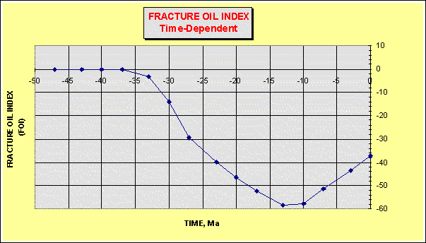
Figure 6 is a plot of the FOI. As presented above, a FOI of less than -1.0 is an indicator of hydrocarbon fracture potential. According to this model, simultaneous and effective oil generation and fracture formation began about 40 Ma at Altamont-Bluebell.

COMPARISON OF UINTA RESULTS WITH A GLOBAL SAMPLE

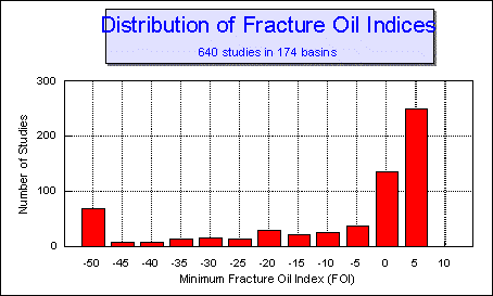
In terms of a relative comparison of FOI from the Uinta Altamont-Bluebell area with a global sample, Figure 7 represents the frequency distribution from 640 case studies distributed in 174 basins. The Altamont-Bluebell example indicates a minimum FOI of -58.3. In the global sample, there are only 61 studies with a FOI less than that found at Altamont-Bluebell. The basins in which the 60 case studies yielded values of less than -58 are:

ALBERTA
ANADARKO
APPALACHIAN
ARABIAN
BENI
CALTANISETTA
CAMPOS
CHACO
GULF COAST
GULF OF VENEZUELA
ILLINOIS
KURA
LOS ANGELES
MARACAIBO
MIDDLE AMAZON
MINCH
NORTH SEA, NORTH
NORTH SEA, SOUTH
PERMIAN
PICEANCE
PO
RATON
RHONE FAN
RIO GRANDE
SACRAMENTO/SAN JOAQUIN
SAN JORGE
SOUTH ADRIATIC
TARANAKI
TARIM
TRANSYLVANIAN
TRINIDAD-TOBAGO
UCAYALI - HUALLAGA
UINTA
VENTURA/ SANTA BARBARA
VIENNA
WEST SIBERIAN
WESTERN OVERTHRUST / BASIN & RANGE
ZAGROS
ZHUNGEER (JUNGGAR)

CONCLUSIONS

1. The fact that the Uinta basin of Utah contains oil and gas in fractured reservoirs makes it an ideal choice location to test a concept that could be used to predict hydrocarbon-rich fractured reservoirs not only in other parts of the Uinta but also in basins in other parts of the world.

2. One can quantitatively predict the simultaneous occurrence of fracture formation and hydrocarbon generation. Such a situation heightens the probability of the fractures remaining open through time, therefore enhancing reservoir potential.

3. Two well-established models can be used to a) predict fracture formation as a function of burial history and b) predict hydrocarbon generation also as a function of burial history.

4. The two models can be combined to produce a unique indicator, called the Fracture Oil Index or FOI. An FOI of less than -1 is an indicator of hydrocarbon-rich fractures.

5. Using EXCEL spreadsheet formats, the calculated minimum FOI for the Eocene Green River Formation in the Altamont-Bluebell field is -58, which occurred 13 Ma at a burial depth of 5.73 km (18,800 ft). The -58 FOI ranks 62 out of 640 in technique-related global studies carried out in 174 basins (60 studies yielded FOI’s less than -58).