^GCPrestack Impedance Inversion Aids Interpretation*

Satinder Chopra¹ and Ritesh Kumar Sharma¹

Search and Discovery Article #41664 (2015)
Posted August 17, 2015

*Adapted from the Geophysical Corner column, prepared by the authors, in AAPG Explorer, June, 2015, and entitled "Impedance Inversion's Value in Interpretation".
Editor of Geophysical Corner is Satinder Chopra ([email protected]). Managing Editor of AAPG Explorer is Vern Stefanic. AAPG © 2015

¹Arcis Seismic Solutions, TGS, Calgary, Canada ([email protected])

General Statement

In Impedance Inversion Transforms Aid Interpretation, Search and Discovery Article #41622 we described the different poststack impedance inversion methods that are available in our seismic industry. In poststack seismic inversion – where there is no mode conversion at normal incidence – it is purely acoustic. P-wave impedance is the only information that can be estimated from poststack inversion of P-wave data. Prestack inversion can be considered when the poststack inversion is not effective enough to meet the desired objectives, such as differentiation of geologic strata or fluid information.

In a seismic gather, the near–offset amplitudes relate to changes in impedance of the subsurface rocks, and thus depict the correct time of the reflection events. The far-offset amplitudes relate to not only the changes in P-wave velocity and density, but the S-wave velocity as well. The inversion of far-offset amplitudes in a gather yields the elastic impedance (as was described in An 'Elastic Impedance' Approach, Search and Discovery Article #41082) and can be used for lithology and fluid discrimination. Thus prestack inversion has an advantage over poststack inversion.

Another significant aspect of prestack impedance inversion is that usually for thin layers in the subsurface, interference effects are reflected as amplitude distortions at different offsets and can be seen after NMO corrections of the seismic gathers. Once the gathers are stacked, however, this information gets lost, and so poststack inversion will not be able to retrieve it. Prestack inversion considers the information in seismic gathers and so is able to provide extra detail, which is not possible with poststack inversion. Prestack seismic impedance inversion also is commonly referred to as simultaneous inversion.

♦General statement
♦Figures
♦Method and Example
♦Conclusions

Figure Captions

	Figure 1. Workflow for simultaneous inversion.
	Figure 2. Three wavelets extracted from the near (blue), mid- (green) and far (light brown) angle stacks, and their amplitude spectra. Notice the frequency content of the wavelet reduces from the near to far angle stack.
	Figure 3a. A portion of a section from P-impedance volume computed using model-based (a) independent inversion, and (b) simultaneous inversion. The yellow, green and light blue arrows indicate the impedance zones (from left to right) that appear much better defined on the simultaneous inversion display in (b) than the independent model-based inversion display in (a).
	Figure 3b. A portion of a section from P-impedance volume computed using model-based (a) independent inversion, and (b) simultaneous inversion. The yellow, green and light blue arrows indicate the impedance zones (from left to right) that appear much better defined on the simultaneous inversion display in (b) than the independent model-based inversion display in (a).
	Figure 4a. A portion of a section from S-impedance volume computed using model-based (a) independent inversion, and (b) simultaneous inversion. The yellow, green, light blue and purple arrows indicate the impedance zones (from left to right) that appear much better defined on the simultaneous inversion display in (b) than the independent model-based inversion display in (a).
	Figure 4b. A portion of a section from S-impedance volume computed using model-based (a) independent inversion, and (b) simultaneous inversion. The yellow, green, light blue and purple arrows indicate the impedance zones (from left to right) that appear much better defined on the simultaneous inversion display in (b) than the independent model-based inversion display in (a).

Method and Example

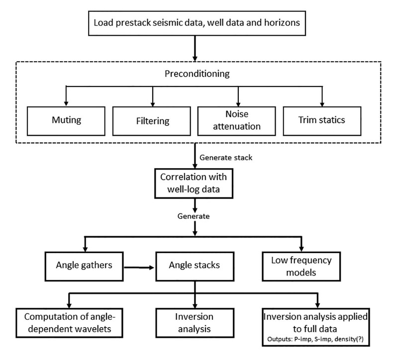
In simultaneous inversion, multiple partial-offset or angle sub-stacks are inverted simultaneously. For each angle stack, a unique wavelet is estimated. Subsurface low-frequency models for P-impedance, S-impedance and density, constrained with appropriate horizons in the broad zone of interest, are constructed, usually with the use of well log data. The models, wavelets and partial stacks are used as input in the inversion, and the output is P-impedance, S-impedance and density. The density attribute is stable and useable, only when large offset/angles are available in the seismic gather.

The workflow shown in Figure 1 explains the different steps followed in simultaneous inversion. The inversion process begins with the low-frequency model, which is used to generate synthetic traces for the input partial stacks. Zoeppritz equations – or their approximations – are used to estimate the band-limited elastic reflectivities. Figure 2 shows the wavelets estimated from the near-, mid- and far-angle stacks for a 3-D seismic volume from the Montney-Dawson area of British Columbia, Canada. The angle-dependent wavelets are convolved with the modeled reflectivities for generating synthetic traces, which are then compared with corresponding real data traces.

The model impedance values are iteratively tweaked in such a manner that the mismatch between the modeled angle gather and the real angle gather is minimized in a least-squares sense. As a different wavelet is extracted for each partial angle stack and used in the inversion, the angle-dependent amplitude information in the gather is utilized.

Not only are the output components useable for interpretation of the physical rock properties, but the quality of the three elastic parameter outputs is enhanced in terms of better resolution. In Figure 3 we show segments of P-impedance sections from the 3-D seismic volume mentioned above:

Figure 3a exhibits a section from the post-stack impedance inversion carried out on the P-reflectivity derived from prestack data. We refer to this as independent inversion.
Figure 3b is the equivalent section from simultaneous inversion.

The stratigraphic column for this area was discussed in Impedance Inversion Transforms Aid Interpretation, Search and Discovery Article #41622.

Shown on the display are the Doig, Halfway (indicated with light blue arrows) and the salt markers (yellow arrows), with shale and siltstone zone (green arrows) in between. Notice that the different zones are defined much better on the simultaneous inversion section as compared with the independent model-based inversion.

Similarly, we show segments of S-impedance sections from the same 3-D seismic volume in Figure 4a and 4b. Again, the definition of the different zones is seen much better defined on the simultaneous inversion display.

Determining Formation Brittleness

The discrimination of fluid content and lithology in a reservoir is an important characterization that has a bearing on reservoir development and its management. Lame's parameter Lambda (λ) is sensitive to pore fluid and is known as a proxy for incompressibility, whereas Mu (μ), the modulus of rigidity, is sensitive to the rock matrix. Referred to as the LMR approach, it consists of determining λρ and μρ from seismic data (as it may be not possible to delink the effect of density (ρ).

Once the P- and S- impedances are determined using simultaneous inversion, they are then used to determine the λρ and μρ attributes. This approach helps in the determination of fluid and lithology in LMR space by way of crossplotting.

For unconventional reservoirs, such as shale resource formations, besides other favorable considerations that are expected of them, it is vital that reservoir zones are brittle. Brittle zones fracture better – and fracturing of shale resource reservoirs is required for their production. Among the different physical parameters that characterize the rocks, Young's modulus (E) is a measure of their brittleness. Attempts are usually made to determine this physical constant from well log data, but such measurements are localized over a small area.

For studying lateral variation of brittleness in an area, 3-D seismic data needs to be used. Computation of Young's modulus from seismic data requires the availability of the density attribute. As stated earlier, the computation of density in turn requires long offset data, which is usually not available.

Conclusion

A new attribute (Eρ) in the form of a product of Young's modulus and density has been introduced, which was discussed in An Effective Way to Find Formation Britleness, Search and Discovery Article #41024. For a brittle rock, both Young's modulus and density are expected to be high, and so the Eρ attribute would exhibit a high value and serve as a brittleness indicator.

The new attribute also can be used for litho-fluid detection, when it is used in conjunction with the product of bulk modulus and density. All this is possible with prestack simultaneous inversion.