GCIntegrated Data Enhance Dolomite Mapping*
Ritsh Kumar Sharma¹, Satinder Chopra¹, and Amit Kumar Ray¹
Search and Discovery Article #41440 (2014)
Posted September 22, 2014
*Adapted from the Geophysical Corner column, prepared by the authors, in AAPG Explorer, September, 2014. Editor of Geophysical Corner is Satinder Chopra ([email protected]). Managing Editor of AAPG Explorer is Vern Stefanic.
¹Arcis Seismic Solutions, TGS, Calgary, Canada ([email protected])
Carbonate sedimentary rocks that have been dolomitized and laterally sealed by tight undolomitized limestone frequently are seen to produce hydrocarbons. The process of dolomitization increases the crystal size and pore size, and thus enhances its porosity and permeability.
As dolomites are less ductile relative to limestones and sandstones, their porosity and permeability also are enhanced by fracturing. Additionally, as they are less reactive than calcites, dolomites are less likely to lose porosity with depth due to dissolution or re-precipitation. For this reason, dolomites often make better reservoirs in carbonates.
Of course the reservoir geometry usually depends on the process of dolomitization and stratigraphic architectures – however, the differentiation between limestones and dolomites is a challenge. The purpose of this article is to describe a workflow for discriminating limestones and dolomites, and to map the lateral extent of dolomite reservoir rocks that have a thickness below the seismic resolution.
|
♦General statement ♦Figures ♦Method ♦Example ♦Conclusion ♦Acknowledgment
♦General statement ♦Figures ♦Method ♦Example ♦Conclusion ♦Acknowledgment
♦General statement ♦Figures ♦Method ♦Example ♦Conclusion ♦Acknowledgment
♦General statement ♦Figures ♦Method ♦Example ♦Conclusion ♦Acknowledgment
♦General statement ♦Figures ♦Method ♦Example ♦Conclusion ♦Acknowledgment |
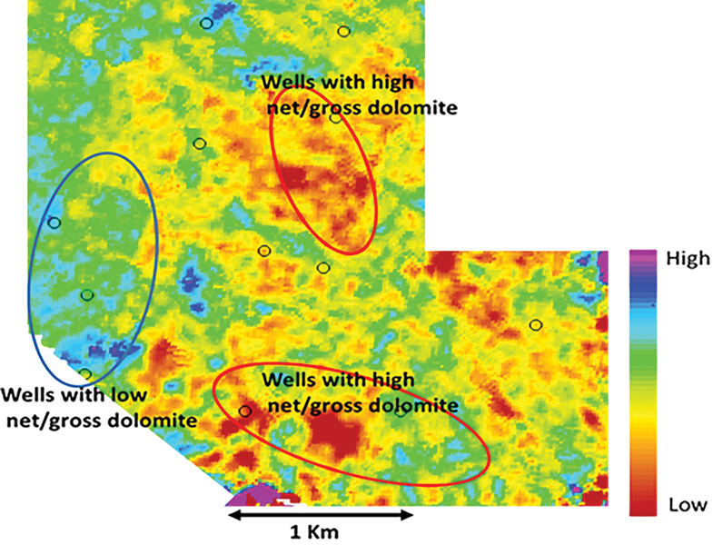
One accepted model for dolomitization is that when hot magnesium-rich brines flow along conduits (faults and fractures) in limestone, hydrothermal dolomites and the associated minerals and fabrics are formed. For the Upper Ordovician Trenton and Black River carbonates in eastern Canada the magnesium required for dolomite precipitation was supplied by magnesium-rich seawater-derived (Silurian and/or Devonian) saline waters from the dissolution of Silurian evaporates. These waters became heated during their descent along faults and fractures to reservoir depths at the center of the basin. Hot basinal brines migrated laterally through basal sandstones, ascended into the network of faults and fractures and precipitated fracture-related dolomite. Compared with clastic reservoirs, the characterization of dolomite reservoirs presents challenges, because many of the conventional methods – comprising attributes such as Lambda-Rho and Mu-rho – are not very effective. Consequently, we need to look for alternative methods for their characterization. While making measurements in the wells (logging), the latest density logging tools make it possible to differentiate between dolomites and limestones using the photoelectric index log. The tool has a gamma ray source that emits the radiation, which enters the formation (about an inch or so), gets scattered and loses energy. The intensity of the back-scattered radiation is picked up by the detectors installed on the tool. While the higher energy part of the backscattered radiation is related to the density, the low energy component is a measure of the average atomic number of the formation or the rock matrix properties (lithology). Fluids have very low atomic numbers, and so have little influence – the limitation, however, is the availability of Pe curves only at well locations. As there is no direct way of computing a 3-D volume of Pe from seismic data, we look for an indirect way of computing it. We demonstrate an integrated workflow in which well data and seismic data from eastern Canada are used to discriminate between limestone and dolomite. The workflow begins with the generation of different attributes from the well-log curves. As shown in Figure 1, using the crossplot between P-impedance and S-impedance, color-coded with Pe values, the blue and red ellipses are drawn corresponding to points that have low and high values of Pe to identify dolomite zones. Instead of using these two separate attributes, it is possible to differentiate between limestone and dolomite by rotating the clusters in a counterclockwise direction. Such a rotation leads to a new attribute, namely lithology impedance (LI), which incorporates lithology formation and can be defined as LI = Ip*sinθ – Is*cosθ, where θ is the angle of the regression line intersection with the horizontal axis (Figure 1). The purpose of generating this attribute (LI) is to be able to use a single attribute for distinguishing the dolomites from limestones. Next, to be able to derive the Pe attribute from seismic data, we investigate the relationship between the LI and Pe well log curves. Such a crossplot is shown in Figure 2, where one can notice a linear relationship in the scatter of points, which are color-coded with density. Such a relationship between LI and Pe curve is deduced from the crossplot and then used for obtaining Pe volume from the seismic data. An important observation one can make from Figure 2 is that LI can be used to distinguish the dolomite from limestone. The dashed blue and magenta lines on this crossplot show the effect of porosity for dolomite and limestone respectively. For deriving these attributes from seismic data, we begin with the prestack seismic gathers. After generating angle gathers from the conditioned offset gathers, the P-reflectivity, S-reflectivity are derived using Fatti's approximation to the As the target dolomite reservoir is thin, it is necessary to enhance the resolution of the seismic data. For this purpose, thin-bed reflectivity inversion (see "Resolving Thin Beds and Geologic Features by Spectral Inversion," Search and Discovery Article #40326 May 31, 2008) was run on the two reflectivities and then filtered back to a bandwidth that is higher than the input data bandwidth. These filtered thin-bed reflectivity data are next inverted into P-impedance and S-impedance. Once these impedance volumes are obtained, it is possible to compute LI. Using the relationship between LI and Pe established from the well, we transform the LI volume into a 3-D volume of Pe, and use that to infer the dolomitic zones. To map the dolomite zones laterally, a horizon slice of Pe volume over a window that includes the zone of interest was generated. A part of that horizon slice is shown in Figure 3. It has been found that throughout the 3-D area the predicted Pe response within the reservoir interval correlates fairly well with the net-to-gross dolomite within the same interval. Rotation of data in P-impedance versus S-impedance crossplot space facilitates the computation of a single attribute known as lithology impedance (LI) that yields information about lithology discrimination within the formation. It was then used to transform the inverted P-impedance volume into a 3-D Pe volume. The derived Pe volume was analyzed, and a fairly good match was seen at the blind wells. It was found that throughout the area covered by the 3-D seismic volume, the predicted Pe response within the reservoir interval correlated fairly well with the net to gross dolomite within the same interval. We thank Arcis Seismic Solutions, TGS, for allowing us to present this work. |