Figure Captions

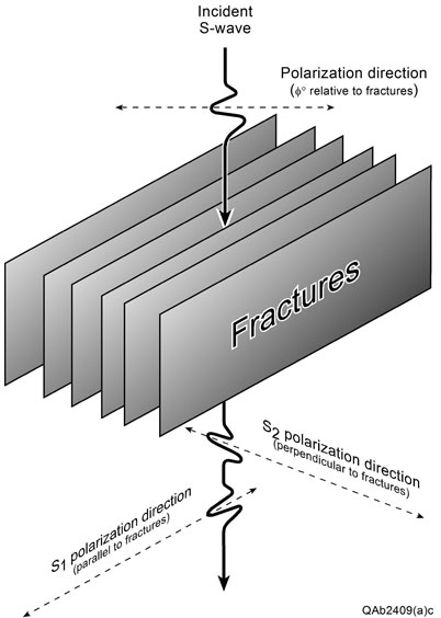	Figure 1. Principles of S-wave splitting in a fractured rock. The incident S wave splits into two components – S1 and S2 – that transmit through a fracture zone and reflect individually from fracture-bounding interfaces. S1 is the fast-S mode, and its particle-displacement vector is oriented parallel to the fracture planes. S2 is the slow-S mode, and its particle-displacement vector is oriented perpendicular to the fracture planes. Reflected modes are not shown.
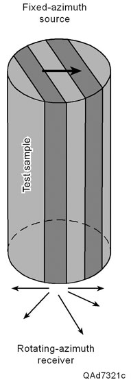	Figure 2. Laboratory measurements of S-wave propagation through a simulated fracture medium.
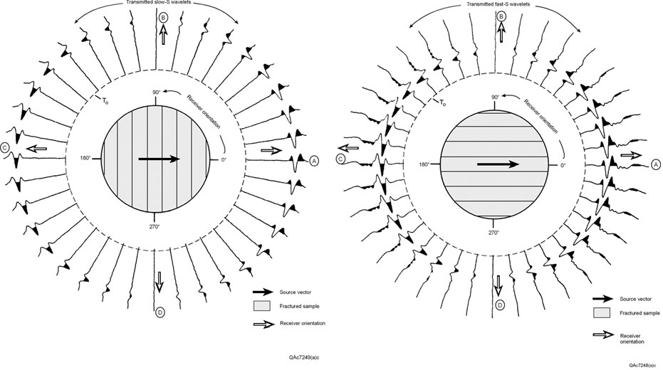	Figure 3. Data acquired using the test arrangement illustrated on Figure 2 to simulate S-wave propagation through a fractured medium. (a) The illuminating S-wave displacement vector is parallel to the test-sample fractures to simulate fast-S propagation. As the source stays fixed on one end of the sample, the receiver at the opposite end of the sample is rotated at angular increments of 10 degrees relative to the positive-polarity orientation of the source displacement vector. Every transmitted response is a fast-S wavelet. The dashed circle labeled T0 defines time zero. Arrowheads define the positive-polarity ends of the source and receiver elements. (b) The same test repeated with the illuminating S-wave displacement vector oriented perpendicular to fractures to simulate the propagation of a slow-S mode. Every transmitted response is a slow-S wavelet. Note how much longer the travel times are for wavelets polarized normal to fractures than they are for the wavelets polarized in 3a that are polarized parallel to fractures.
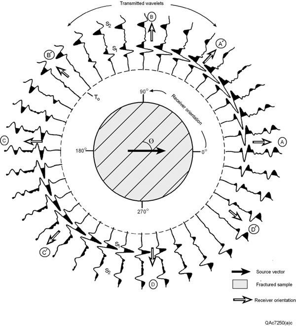	Figure 4. End-on view of a fractured test sample from the source end. The source vector is polarized at an angle Φ relative to the azimuth of the fracture planes. As the source remains fixed at one end of the test sample, the receiver at the opposite end is rotated 360 degrees at angular increments of 10 degrees relative to the orientation of the positive-polarity of the S-wave source vector. These test data show that only a fast-S (or S1) mode propagates parallel to fracture planes (responses A’ and C’), and only a slow-S (or S2) mode propagates perpendicular to the fracture planes (responses B’ and D’). A mixture of S1 and S2 is observed at all other azimuth orientations. Amplitude behavior is affected by the continually changing angle between the vector orientations of the positive-polarity ends of the source and receiver elements. Dashed circle T0 defines the travel time origin T=0 for the wavelets. Modified from Sondergeld and Rai (1992).
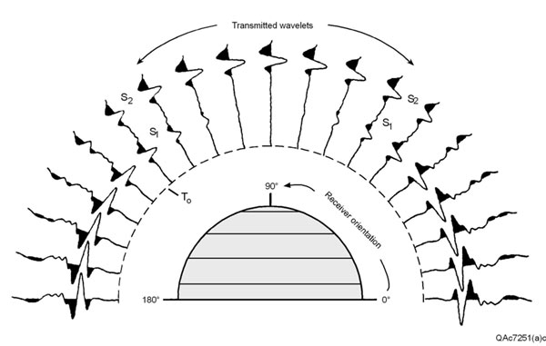	Figure 5. S-wave propagation through a fracture system observed when the source and receiver are aligned in the same azimuth, as is done when processing actual S-wave seismic data. S1 is the fast-S mode. S2 is the slow-S mode. The azimuth angle in this graphic defines the orientation of the positive-polarity end of both the source and receiver relative to the fracture planes, whereas the angle in previous figures defines the orientation of the receiver relative to the source. Only S1 propagates parallel to fractures, and only S2 propagates perpendicular to fractures. Modified from Sondergeld and Rai (1992).
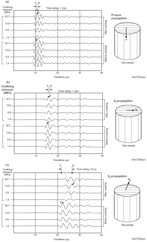	Figure 6. Travel time measurements through a test sample before (bottom four traces) and after (top four traces) cracking the sample to create a propagation medium of quasi-aligned fractures. Confining pressure was varied as labeled between measurements. A principal finding is that P and S1 react weakly to the presence of fractures (panels a and b), but S2 reacts strongly (panel c). Modified from Xu and King (1989).
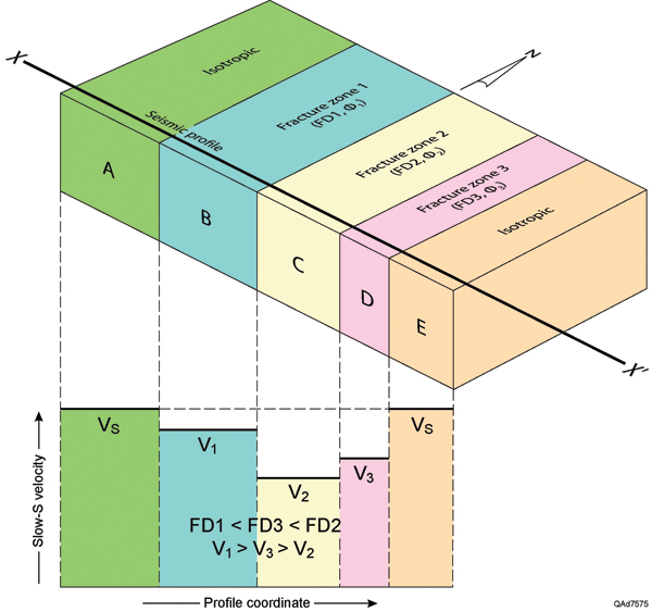	Figure 7. Relationship between slow-S velocity (S2) and fracture density (FD). As fracture density increases, S2 velocity decreases. In contrast, fast-S velocity S1 and P-wave velocity VP do not change, or change by only minor amounts across blocks A through E. In isotropic blocks A and E, there is no S-wave splitting and only one S-wave velocity VS. In all blocks (A through E), fast-S velocity = VS, the velocity in the non-fractured rock. Mineralogy, porosity and pore fluid do not change across the profile. The only Earth properties that vary from block to block are fracture density and orientation.
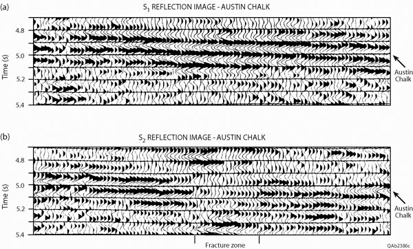	Figure 8. S1 and S2 images along a profile that traverses an Austin Chalk play. The S2 chalk reflection (b) is delayed by about 50 ms relative to the S1 reflection (a) because of the difference in S1 and S2 propagation velocities through the overburden above the chalk. From well control, it was determined that fracture zones occur where the S2 chalk reflection dims but the S1 reflection does not. Such S2 dimming is expected across fracture trends because S2 velocity in a zone of higher fracture density slows to almost equal the S-wave velocity in the top seal above the chalk. Data published by Mueller (1992).
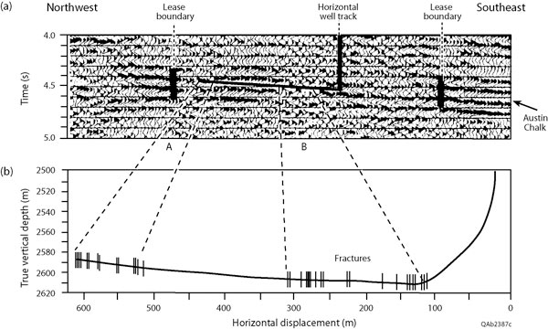	Figure 9. (a) S2 reflection profile across an Austin Chalk lease. The coordinates followed by the vertical and horizontal legs of an exploration well are superimposed on the seismic image, as are the locations of the lease boundaries. (b) Fractures found along the horizontal leg of the well were concentrated in the two zones, A and B, where the S2 reflection dimmed. Laboratory data discussed in preceding articles infer S2 velocity lowers (and thus S2 reflectivity decreases) when fracture density increases. That principle is now put into exploration practice. Data published by Mueller (1992).
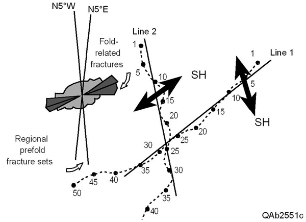	Figure 10. Fracture orientation across a prospect area and two crooked-line profiles (the dotted lines) used to evaluate fracture attributes. The solid lines show the position of the images created by crooked-line processing. Arrows labeled SH define the polarization of the SH particle-displacement vector on each seismic line. An older, pre-fold fracture set is oriented north-south; a younger and more dominant fold-related fracture set is oriented east-west. Line 1 follows the orientation of the dominant younger fractures. The SH displacement vector along Line 1 is the slow-S mode for the younger fractures. Line 2 follows the trend of any north-south fractures that may be present. The SH displacement vector along Line 2 will be the fast-S mode for the younger, dominant, pre-fold fractures. Modified from Alford and others (1989).
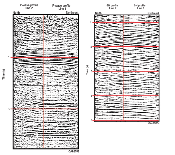	Figure 11. (a) Comparison of P-wave images. All events are time aligned at the tie point, showing that, at this location, P-wave velocity is invariant perpendicular and parallel to fractures. (b) Comparison of SH images. Reflections on Line 1 occur at later times than do corresponding reflections on Line 2 because of the wave-propagation physics of fast-S and slow-S modes through the dominant, younger fracture set that extends across most of the overburden above the fracture target. Modified from Alford and others (1989).
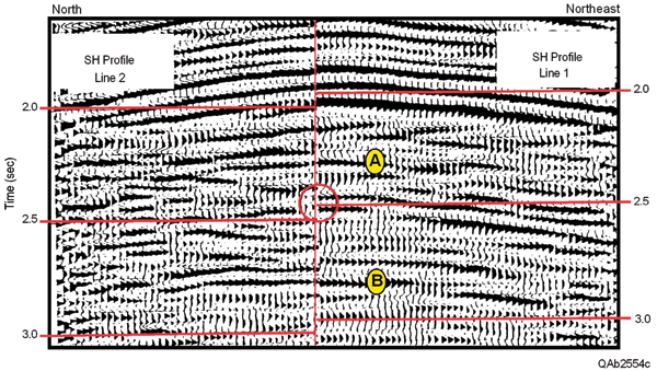	Figure 12. Comparison of event-aligned SH images across the targeted sandstone reservoir. The SH image on Line 1 is advanced in time so that there is a reasonable alignment of events A and B that span the reservoir interval, the interval circled at 2.5 s. Within this circled data window, the dimming on Line 2 means that the SH polarization on Line 2 is the slow-S mode for the fracture target. Because the SH polarization on Line 2 is east-west (Figure 10), then north-south fractures must be present within the reservoir interval for SH motion on Line 2 to be a slow-S mode. Modified from Alford and others (1989).

S-Wave Splitting Phenomenon

S-wave splitting phenomenon is illustrated on Figure 1, where an S wave illuminates a zone of well-aligned vertical fractures. The incident S wave is polarized so that its particle-displacement vector is oriented at an angle Φ relative to the azimuth of the vertical fractures. S1 and S2 modes exit the base of the fracture zone at different times because they propagate with different velocities inside the fracture space (S1 = fast; S2 = slow). As expected, the S1 mode is polarized parallel to the fracture planes, and the S2 mode is polarized perpendicular to the fracture planes. S1 and S2 modes also reflect from the fracture zone, but are not shown.

A laboratory test that documents the S-wave physics described by this model was published by Sondergeld and Rai (1992). Their test procedure is illustrated on Figure 2. In this test, a piezoceramic element was secured to one end of a cylindrical volume of laminated shale to serve as an S-wave source. A similar piezoceramic element was positioned at the opposite end of the cylinder as an S-wave sensor. This layered propagation medium, and the fact that the source-receiver geometry causes S-waves to propagate parallel to the embedded interfaces of the rock sample, are a good simulation of S-wave propagation through a system of vertical fractures.

In one test, the source remained in a fixed orientation relative to the plane of the simulated fractures and the receiver element was rotated at azimuth increments of 10 degrees to determine the azimuth dependence of S-wave propagation through the sample. The test results are illustrated on Figure 3 as an end-on view of the test sample from the source end; the objective was to simulate the propagation of a fast-S (or S1) mode, where the source displacement vector is parallel to the fracture planes (Figure 3a), and then to simulate the propagation of a slow-S (or S2) mode in which the displacement vector is perpendicular to the fracture planes (Figure 3b). Note how much longer it takes for the S2 wavelet to propagate through the test sample than the S1 wavelet – a confirmation that S2 velocity is slower than S1 velocity.

The positive-polarity end of the source is oriented in the direction indicated by the arrowhead on the source vector. For response A, the positive-polarity of the receiver is oriented the same as the source. For response C, the receiver has been rotated so that its positive-polarity end points in an opposing direction. Thus the polarity of wavelet B is opposite to the polarity of wavelet A.

In actual seismic fieldwork with S-wave sources and receivers, the positive polarities of all receivers are oriented in the same direction across a data-acquisition template so that wavelet polarities are identical in all quadrants around a source station. At receiver orientations B and D, the receiver is orthogonal to the source vector, which produces zero-amplitude responses.

The translation of these experimental results into exploration practice means that seismic prospecting across fracture prospects should involve the acquisition of S-wave data – and further, the data-acquisition geometry should allow S-wave velocity to be measured as a function of azimuth. When an azimuth direction is found in which S velocity across the depth interval of a fracture system has its maximum velocity, then the orientation direction of the dominant vertical fracture in that interval is defined as that maximum-velocity azimuth.

S Waves Laboratory Experiments on Real-Earth Media

Now we expand our insights into the behavior of seismic S waves as they propagate through a fractured interval, with the emphasis placed on laboratory data of real S waves propagating through fractured real-Earth media. The experimental data illustrated on Figure 4, taken from work published by Sondergeld and Rai, simulate the general case of S-wave illumination of a fracture system in which the illuminating source vector is polarized at an arbitrary angle Φ relative to aligned fractures. The test sample used to acquire the data was illustrated and discussed above.

The wavefields that propagate through the medium are now a combination of S1 (fast-S) and S2 (slow-S) wavelets, and not S1-only or S2-only wavelets as were generated in the experimental data discussed above. Wavelets A, B, C and D are again the responses observed when the receiver is either parallel to or orthogonal to the illuminating source vector. The observed data contain both S1 and S2 arrivals. The length of the propagation path through the sample is such that the difference in S1 and S2 travel times causes the S1 and S2 wavelets to not overlap.

In real seismic data, when a fracture interval is thin compared to a seismic wavelength and the difference in S1 and S2 travel times is not too large, the response will be a complicated waveform representing the sum of partially overlapping S1 and S2 wavelets. The wavelets at positions A', B', C' and D' illustrate important S-wave physics:

• Only a S1 mode propagates parallel to the fracture planes (responses A' and C').
• Only a S2 mode propagates perpendicular to the fracture planes (responses B' and D').

The experiment documented as Figure 5 illustrates the results that should be observed when S-wave data are acquired across a fracture system as a 3-D seismic survey in which there is a full azimuth range between selected pairs of sources and receivers. In this test, the source and receiver are rotated in unison so that the positive-polarity ends of both source and receiver are always pointing in the same azimuth. This source-receiver geometry is what is accomplished during S-wave data processing when field data are converted from inline and crossline data-acquisition space to radial and transverse coordinate space that allows better recognition of S-wave modes.

This type of source and receive r rotation is common practice among seismic data processors that have reasonable familiarity with S waves. The test data show convincing proof that only a fast-S mode propagates parallel to fractures, and only a slow-S mode propagates perpendicular to fractures. At all intermediate azimuths between these two directions, S-wave propagation involves a mixture of fast-S and slow-S wavefields.

The objective of real-Earth fracture evaluation is to acquire seismic data in a way that allows source and receiver rotations to be done to create data similar to that shown on Figure 5. These rotated data are then searched to find the azimuth direction in which S-wave velocity is a maximum. That maximum-velocity azimuth defines the orientation of the set of vertical fractures that dominate the fracture population.

P, S1, S2 Wave Laboratory Behavior: Cracked vs. Uncracked Rock

Experimental work done by Xu and King (1989) are presented as Figure 6. In this lab experiment, P, S1 (fast-S) and S2 (slow-S) modes propagate through a test sample before and after the sample was cracked to create a series of internal fracture planes. Wave transit times through the sample were measured to determine the effect of cracks on the velocity of each wave mode.

For both the cracked and uncracked samples, transit time measurements were made for a series of confining pressure conditions varying from 1.4 MPa to almost 21 MPa. P-wave travel time behavior is described on the top panel of the figure; S1 and S2 travel times are summarized on panels b and c, respectively. On each data panel, the transit time for uncracked rock is marked as A. Point B indicates the travel time through the cracked sample.

The travel times for P and S1 modes exhibit little pressure dependence over the applied pressure range for either cracked or uncracked media. There is a noticeable decrease in transit time for the S2 mode as confining pressure is increased. This behavior is indicated by the dashed line drawn across the S2 waveforms on panel c.

The wave physics confirmed by this test is that P and S1 velocities decrease by only a small amount – often a negligible amount – when a seismic propagation medium changes from non-fractured rock to a medium with aligned-fractures. The observed delay in transit time through the small test sample is less than 2 µs for each of these wave modes when fractures are present. In contrast, the delay in travel time for the S2 modes exceeds 5 µs – more than twice the transit-time delays of the P and S1 modes. Data point B for the S2 mode propagating in the cracked rock is arbitrarily selected from the waveform observed at the mid-pressure range used in the test.

Earth System Model

Physical measurements of S-wave transit time through fractured media – such as those documented on Figure 6 – establish the relationship between slow-S velocity and fracture density illustrated on Figure 7. This model simulates a seismic profile traversing an Earth system consisting of blocks of anisotropic rock bounded by blocks of isotropic rock. Anisotropic conditions in blocks B, C and D are caused by aligned fractures that have different fracture density (FD) and fracture azimuth (Φ) from block to block.

When this Earth system is illuminated with an elastic wavefield, slow-S velocity has the generalized behavior diagramed below the Earth model. As fracture density FD increases, slow-S velocity S2 velocity decreases. The magnitude by which S2 decreases is a qualitative, not quantitative, indicator of fracture density. S2 velocity behavior can be used to predict fracture density in a quantitative manner only if fracture density can be independently determined at several calibration points across seismic image space – and establishing such calibration is difficult.

Restricting the use of S2 velocity behavior to that of only a qualitative predictor of fracture density is still important and valuable for understanding fracture distribution across areas imaged with multicomponent seismic data. Variations in fracture azimuth Φ affect only the polarization direction of the slow-S mode, not the magnitude of S2 velocity.

Fast-S velocity in a fractured medium is approximately the same as it is in an unfractured sample of that same medium (Figure 6b). S1 velocity may decrease by a small amount if fracture density is sufficient to alter bulk density; otherwise, it is reasonably correct to assume S1 has the same magnitude in fractured rock as it has in non-fractured sections of the same rock.

Measuring Factures – Quality and Quantity

As has been emphasized in the three sections of this series, when a shear (S) wave propagates through a rock unit that has aligned vertical fractures, it splits into two S waves – a fast-S (S1) mode and a slow-S (S2) mode. The S1 mode is polarized in the same direction as the fracture orientation; the S2 mode is polarized in a direction orthogonal to the fracture planes.

Here we translate the principles established by laboratory experiments discussed in the preceding sections of this series into exploration practice.

Figure 8 displays examples of S1 and S2 images along a profile that crosses an Austin Chalk play in central Texas. The Austin Chalk reflection in the S2 image occurs later in time than it does in the S1 image because of the velocity differences between the S1 and S2 modes that propagate through the overburden above the chalk. Subsurface control indicated fractures were present where the S2 chalk reflection dimmed but the S1 reflection did not.

This difference in reflectivity strength of the S1 and S2 modes occurs because when fracture density increases, the velocity of the slow-S mode becomes even slower. In this case, the S2 velocity in the high-fracture-density chalk zone reduces to almost equal the S-wave velocity of the chalk seal, which creates a small reflection coefficient at the chalk/ seal boundary.

When fracture density is small, S2 velocity in the chalk is significantly faster than the S-wave velocity in the sealing unit, and there are large reflection coefficients on both the S1 and S2 data profiles.

Using this S-wave reflectivity behavior as a fracture-predicting tool, a horizontal well was sited to follow the track of a second S2 profile that exhibited similar dimming behavior for the Austin Chalk. The S2 seismic data and the drilling results are summarized on Figure 9. Data acquired in this exploration well confirmed fractures occurred across the two zones A and B where the S2 reflection dimmed and were essentially absent elsewhere.

The seismic story summarized here is important whenever a rigorous fracture analysis has to be done across a prospect. If fractures are a critical component to the development of a reservoir, more and more evidence like that presented here is appearing that emphasizes the need to do prospect evaluation with elastic-wavefield seismic data that allow geology to be imaged with both P waves and S waves.

The value of S-wave data is that the polarization direction of the S1 mode defines the azimuth of the dominant set of vertical fractures in a fracture population, and the reflection strength of the S2 mode, which is a qualitative indicator of S2 velocity, infers fracture density.

The Earth fracture model assumed here is a rather simple one in which there is only one set of constant-azimuth vertical fractures. What do you do if there are two sets of fractures with the fracture sets oriented at different azimuths?

Detecting Two Separate Sets of Fractures

In areas where fracture-producing stress fields have been oriented at different azimuths over geologic time, there can be fracture sets of varying intensities and different orientations across a stratigraphic interval. Here we consider how to use shear (S) seismic data to locate a fracture set oriented at a specific azimuth in a target interval that is embedded in a thick section dominated by a younger and more dominant fracture set oriented in a different azimuth.

The fracture orientations and two crooked-line surface profiles where compressional (P) and S-wave seismic data were acquired are illustrated on Figure 10.

Two fracture trends are present:

• An older, pre-fold fracture set oriented approximately north-south.
• A younger, more dominant set, oriented approximately east-west, produced during a regional orogeny that fractured massive intervals of rock.

The older fractures can be open and gas-filled in a targeted unit at a depth of approximately 10,000 feet (3,000 meters). The objective is to find this relatively thin interval with a north-south fracture set embedded in a thick section of more dominant, fold-related, and nonproductive east-west fractures.

P-wave and SH-wave seismic data acquired along the two crooked-line profiles are shown as Figure 11. The P-wave profiles tie at their intersection point, showing that P waves exhibit minor difference in velocity when they propagate parallel to and orthogonal to the east-west fractures that extend across a large part of the geological section. This weak reaction of P-wave velocity to fracture orientation is one reason why P-waves have limited value for analyzing fracture systems.

A different behavior is observed for the SH data. SH reflections on Line 2, where the SH particle-displacement is aligned with the dominant east-west fractures (Figure 10), arrive earlier than do their corresponding reflections on Line 1, where the SH particle-displacement vector is orthogonal to the extensive east-west fractures.

As has been described in the preceding sections of this series, the SH polarization along Line 2 is the fast-S mode for the east-west fractures, and the SH polarization along Line 1 is the slow-S mode for east-west fractures. By comparing these P and SH images, we see hard evidence that S-wave velocity reacts more strongly to fractures than does P-wave velocity.

A valuable interpretation procedure is illustrated on Figure 12, where the two SH profiles are depth registered across the reservoir target interval. Here, the image on Line 1 is advanced in time to align key reflection events A and B above and below the targeted reservoir, the circled event at the tie point. If the desired north-south fractures are present within the reservoir interval, the reflection event will dim on Line 2, because the SH polarization on that profile would be the slow-S mode for a north-south fracture set.

As shown in above sections, slow-S velocity S2 decreases when fracture density increases, and thus S2 reflectivity weakens as shown in this example. In contrast, the reflection would remain bright on Line 1, where the SH polarization is the fast-S mode for north-south fractures. That reflectivity behavior is what is demonstrated inside the circled target interval.

The exploration problem described here of locating a subtle fracture set hidden by a more dominant fracture set is one of the most challenging that can be encountered in interpreting fracture attributes from seismic data. The fundamental principle illustrated by this case history is that multicomponent seismic data that provide both P and S data are far more valuable for fracture analysis than are single-component P-wave data alone. Incidentally, this story and its illustrations are taken from a 20-year old U.S. patent (#4,817,061) – showing that good technology can be found in places other than technical journals.

References

Alford, R.M., L.A. Thomsen, and H.B. Lynn, 1989, Seismic surveying technique for the detection of azimuthal variations in the Earth’s subsurface: US patent #4817061, filed 3/28/89, 29 pp., Web accessed 8 August 2011, http://www.google.com/patents

Mueller, M.C., 1992, Using shear-waves to predict lateral variability in vertical fracture intensity: Geophysics-The Leading Edge of Exploration, v. 11/2, p. 29-35.

Sondergeld, C.H., and C.S. Rai, 1992, Laboratory observations of shear-wave propagation in anisotropic media: Geophysics-The Leading Edge of Exploration, v. 11/2, p. 38-43.

Xu, S., and M.S. King, 1989, Shear-wave birefringence and directional permeability in fractured rock: Scientific Drilling, v. 1/1, p. 27-33.

Return to top.

 

Copyright © AAPG. Serial rights given by author. For all other rights contact author directly.