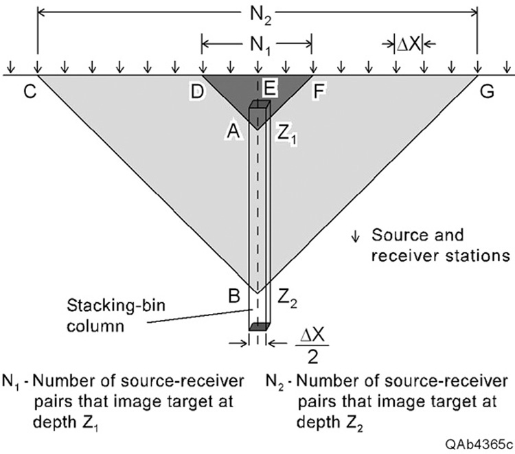
Figure 2. Vertical variation in stacking fold. The source-station and receiver-station spacings along this profile have the same value Δx, which results in a stacking bin width of Δx/2. The vertical column shows the coordinate position of one particular stacking bin. For a deep target at depth Z2, the stacking fold in this bin is a high number because there is a large number (N2) of source-receiver pairs that produce a raypath that reflects from subsurface point B. Only one of these raypaths, CBG, is shown. For a shallow target at depth Z1, the stacking fold is low because there is only a small number (N1) of source-receiver pairs that produce individual raypaths that reflect from point A. One of these shallow raypaths, DAF, is shown. When a 3-D seismic data volume is described as a 20-fold or 30-fold volume, people are usually referring to the maximum stacking fold that is created by the 3-D geometry, which is the stacking fold at the deepest target.