Click to
view article in PDF format (~5.3 mb).
Click to
view article in PDF format (~5.3 mb).
Seismic Stratigraphy-A Primer on Methodology
By
John W. Snedden1, and J. F. (Rick) Sarg2
Search and Discovey Article #40270 (2008)
Posted January 19, 2008
1ExxonMobil Upstream Research Company, Houston, Texas ([email protected])
2Colorado Energy Research Institute, Colorado School of Mines, Golden, Colorado ([email protected])
Seismic stratigraphic methods allow one to interpret and map reservoir, source, and seal facies from reflection seismic data. Seismic stratigraphic methods have evolved since the first publications in the late 1970’s. This document attempts to provide an update of these elementary principles, written as a “how-to” series of steps.
|
|
Seismic stratigraphic techniques have evolved considerably since the underlying principals were first discussed over twenty years ago (e.g. Vail et al., 1977). Seismic stratigraphy methodology has proven quite successful in identifying plays on a regional basis, maturing leads to drillable prospect status, and exploiting field hydrocarbon resources (Greenlee, 1992; Duval et al., 1992). In this document, we discuss some guidelines for conducting a seismic stratigraphic investigation and include guidelines for data preparation. This type of work should lay the foundation for later sequence stratigraphy (Van Wagoner et al. 1988), seismic attribute analysis (2D or 3D), volume interpretation (3D), and forward seismic and geological modeling. However, these recommendations are meant to form a working approach rather than a series of subjective directions. Methodologies must always be adjusted to fit the data from a given area. Further reading is listed to support the information provided here.
As regional seismic stratigraphic analysis often proceeds detailed 3D seismic mapping, it is assumed that the first stages of analysis involve 2D seismic or merged 2D/3D datasets with relatively long lines (>1-5 km line length). Preparing these data for analysis usually require the following six steps: 1. Plot regional base maps showing shot points and posted wells. These should be at an appropriate scale and size for later use in mapping. Bathymetry is also useful to have in offshore datasets. Base maps serve several functions, including places to mark seismic facies notations, areas of interest, anomalies to further investigate, checking line ties, etc. 2. From the base map, select key 2D or 3D seismic lines, emphasizing regional or sub-regional dip lines with important well-ties. Avoid, if possible, areas where wells must be extrapolated considerable distances (> 1 km) along strike or down structural dip to tie seismic lines. Select lines to allow loop ties in a progressively widening grid, avoiding severe tectonic deformation zones, if possible. Identify possible "hero" lines, often dip lines, which tie key wells and show clear stratigraphic trends and are good "show lines". Sometimes the best choices for hero lines emerge later on, following initial interpretation. 3. Plot paper copies of selected regional seismic lines at a reduced scale. We highly recommend using wiggle trace paper sections at the first stages of an investigation as this is usually the best way to see complex stratal relationships and terminations over long distances (Table 1). On the seismic workstation, such stratal observations are often obscured or masked by a high degree of vertical exaggeration. Long regional lines often require panning large back and forth on a workstation, whereas paper sections allow uninterrupted visual scanning for key terminations. In addition, wiggle trace sections, which allow for marking of often subtle stratal terminations, do not display well on the workstation screen. Figures 1 and 2 illustrate the results of plotting a small portion of a seismic workstation view with wiggle trace and variable density displays at regional scales (1:50,000). Notice how onlap of the seismic reflections is more clearly displayed on the wiggle trace section (Figure 1) than the variable density plot (Figure 2). This also holds true for the prospect or field scale at 1:25,000 (Figures 3 and 4). Variable density sections (as on seismic workstations) are more difficult to interpret stratigraphically than wiggle trace (variable area) sections because stratal terminations tend to be “smoothed out” by this type of display. In addition, the subtle brightening of adjacent reflections at a stratal termination, due in part to tuning effects, is often masked. If there is a desire to make the troughs stand out more, one can color these with a light shade of gray for greater contrast. 4. Avoid data which has trace-mixing that obscures stratal terminations. Avoid narrow AGC (automatic gain control) windows which tend to reduce differences in relative amplitude between stratigraphic units. Use migrated sections where possible, but this is not a requirement (sometimes non-migrated data is better for seismic stratigraphic interpretation).
5. Prepare well data for seismic
ties. We recommend that well ties be made paper to paper in the
early 1) Identifying a key reflection (typically a limestone/shale contact) with high acoustic impedance contrast and hanging the synthetic on it. 2) In some cases with limited or older velocity data, there is some utility in constructing a time-depth (T-Z) curve for the region using other checkshot surveyed wells. This empirical approach often yields a polynomial equation to predict depths from seismic TW time. Most check-shot data can be fit with a second-order polynomial (y = 2x +b) where y is depth and x is TW time. Be careful of areas where overpressuring causes variations in T/Z plots. Keep in mind that some bulk time-shifting can still be required to match the seismic (generally less than 100 ms). 6. We highly recommend construction of a well-tie template for illustrating the relationship between seismically-defined surfaces, time-based well log, biostratigraphic calibration, and global chronostratigraphy. This template can be prepared once horizons have been identified and well-ties are made with general agreement among interpreters. It also useful for project presentations as it provides a clear documentation of the stratigraphic age model used.
Seismic Stratigraphy Interpretation Once data has been properly prepared, seismic stratigraphic interpretation begins, typically using colored pencils for different horizons. While the speed and ease of work-station correlation is far greater than hand interpretation, there always is a basic need to develop regional ‘hero lines” to illustrate key stratigraphic relationships. Having a hero line or series of hero lines is a useful way of reducing variations among interpreters, as these become the starting point for any new seismic workstation project. Pencil-interpreted paper sections allow for some changes in correlation, especially when looping across other sections occurs. However, at some point the lead interpreter declares that the key horizons are “looped” and only limited significant subsequent alterations are allowed.
Interpretation Steps 1. Identify areas of major structural deformation and data artifacts (sideswipe and diffraction) on the seismic sections. One should have a sense of the general tectonic style, presence of structural decollements, or key deformational events from previous reports or the literature. Do not blindly adhere to conventional wisdom if seismic data dictates otherwise. 2. In structurally complex terrains, it may be useful to do an initial correlation of a few surfaces and then cut, flatten, and tape together sections to see key tectonic relationships. A few half-scale seismic displays at or near 1:1 vertical exaggeration may also be helpful if structure is not clear-cut. Interpret faults (with normal pencil) where obvious offsets can be identified. Be sure to differentiate between migrated and unmigrated seismic sections where identifying faults. Also be careful of pitfalls due to over- or undermigration of seismic data. In some cases, complete restoration of a series of seismic sections is necessary to fully understand the original depositional patterns and stratigraphic organization (e.g. Gulf of Mexico slope salt province). 3. Review key lines (especially dip lines) to identify major (second-order) shelf margins, if present in the region. Indicate by triangle or circular symbol. Get a feel for the scale of the seismic sequences (2nd order, 3rd order, etc.), and pre-, syn-, and post-orogenic sequences. Identify major angular truncations by bold top truncation arrows (in red). 4. Begin to identify major lapouts with red pencil marks. Do this BEFORE making seismic correlations. Stratal terminations are listed in order of importance and illustrated in Figure 5: -angular truncation obvious erosional termination of dipping reflections up against a reflection of lesser dip) -onlap (stratal termination up against a reflection of greater dip) -downlap (stratal termination down against a reflection of lesser dip) -toplap (termination of successively younger reflections against a reflection, passing downdip to prograding clinoforms (in some cases))
5. Connect onlap and angular truncation terminations as a candidate sequence boundary. Connect the downlaps as a candidate maximum flooding surface (MFS), keeping in mind the caveats listed above. Toplaps remain unconnected temporarily. Be careful when interpreting onlaps and downlaps in strike sections or in tectonically rotated and growth fault sections. Please note that listric fault planes or glide planes can be misinterpreted as onlaps.
6. Keep in mind that the most
important seismic stratigraphic surface is the sequence
boundary (SB), which is most easily identified by stratal
onlap, especially in shelfal portions of the sequences. It will
be most continuous throughout the area of interpretation. Both
toplap and downlap surfaces can change reflection position for
various reasons. For example, the toplap surface can drop below the
sequence boundary in a lowstand
7. Look in basinal positions for
double downlap as an indicator of LST-basin-floor thick or (in
slope) slope thicks or channels. The sequence boundary on the basin
floor is by definition a correlative conformity and may not
necessarily show much associated erosion. However, in confined
deepwater channel
8. Look in shelf-margin position for LSW’s, which will often be
indicated by detached, shingled toplap-downlap couplets. These
should be colored separately from other 9. Carry through the correlations made by connecting stratal terminations marks. Loop-tie the sequence boundary (SB) and maximum flooding surface (MFS) in a progressively widening set of line ties, in order to gain confidence in the correlations. At least five or more surfaces need to be tied in multiple loops before correlations are considered more than “candidate” SB or MFS.
10. A good practice in seismic
stratigraphic correlation is to drag your pencil on the black peak
or at the zero crossing just above the peak. One reason for this is
the ease in erasing the pencil line should a miss-tie occur.
However, if the impedance characteristics of sand and shale are
well established and the surface type and position are known, it is
more important to correlate the surface in the appropriate peak or
trough. Knowing whether seismic data is quadrature or zero 11. A general rule of thumb when correlating, either with pencil or with workstation cursor, is to stay low as possible without crossing reflections when correlating a SB in the basin. Conversely, it is wise to stay high when correlating on the shelf, without crossing reflections. A MFS surface may rise in the basin (due to sedimentation prior to downlap). As mentioned, low toplap is common and can be confused with a sequence boundary but may be an internal surface in the LSWpc. This is why it is so important to understand the type of surface that is being correlated and the basin position of the area being interpreted.
Integration with Other Data Types After key stratigraphic surfaces have been identified and correlated, the next set of steps are undertaken to integrate any available well data. 1. Integrate with logs, cores, and biostratigraphic information. --Biostratigraphic data: It is important when using biostratigraphic data to look for concentration/dilution cycles. In general terms, concentration cycles, zones where large numbers of microfauna and flora are condensed over short intervals, are often associated with maximum flooding surfaces (MFS). By contrast, dilution cycles are often associated with sequence boundaries. Keep in mind the potential for depressed fauna and displaced (transported) fauna. Be careful where data comes from wells with thin stratigraphic sections on structural or paleogeographic highs. Sequence boundaries sometimes are associated with high numbers of reworked older fauna, usually due to updip or local erosion of older strata. Biofacies and paleoclimatic inferences from paleontologic data should also be considered in this integration because latitude variations in faunal and floral content can also occur (Armentrout et al., 1991). --Logs: Stacking patterns, log motifs, and lithology are keys to the intermediate scale of correlation which should support the seismic correlations. In fact, the best log correlations are established when the seismic data is used as a guide to extending stratigraphic surfaces from well to well. While seismic data does not often capture the high-resolution stratigraphic correlations possible in a log cross-section, it usually displays gross geometries (e.g., dipping clinoforms) which should be followed in log correlation. For example, experience has shown that clinoforming parasequences or stacked sequence architectures can be missed in log correlation if not first identified on seismic. Stacking patterns seen on logs (and outcrops sections) are often indicative of key stratigraphic surfaces. For example, the change from retrogradational to progradational stacking often is associated with a maximum flooding surface, which can be checked against both seismic and biostratigraphic data.
Log motif interpretation of
--Lithologic relationships
can help identify --Cores: The best evidence for identification and validation of important stratigraphic surfaces often comes from cores. Sequence boundaries can be associated with basal lags or paleosols (on the interfluves of incised valley-fills (ivf’s)). Parasequence boundaries (PSB’s) can be associated with burrowed, wave rippled surfaces. The Glossifungites trace fossil assemblage is a firm or hard ground indicator and this can be associated with PSSB or PSB’s. At this point, it is often helpful to take some of the sequence boundaries and maximum flood surfaces from the sequence stratigraphically interpreted seismic sections and post these on log cross-sections. The result is seismic-consistent well log correlation (as described in item #1). Such sections are good ways to illustrate how seismic geometries point to sand type, thickness, and distribution (shelf vs. basin, for example). Of critical importance is the need to pick a surface that is a good (flat) datum. The surface chosen should have been close to horizontal at the time of deposition. This is not easy, considering that virtually every surface has some stratigraphic dip. If the surface elevations are close, then perhaps hanging on subsea depth might work. Maximum flooding surfaces often work well in basinal settings while shelf top sequence boundaries in shelfal domains are favored. Flooding or transgressive surfaces work well locally, but are clearly diachronous at the regional scale. Once surfaces are established, it is relatively easy to compute statistics like net/gross, etc., used in map overlays described below. Multiple datums may be necessary, particularly with long regional cross-sections, but many computer cross-section programs have some difficulty with this.
2.
Color 3. Use biostratigraphic information to date the sequence boundaries and MFS. It is very important to establish sequence boundaries ages at the narrowest lacuna (smallest hiatus). This is particularly critical for major angular or structural unconformities (e.g., Middle Miocene Unconformity (MMU) of SE Asia, Base Cretaceous in Northern Viking Graben). Figure 6 illustrates how the MMU of Malaysia was definitively dated at 15.5 ma (Haq et al., 1987 terminology) by using biostratigraphic age dates where the gap between the oldest strata above and the youngest strata below the MMU was identified. 4. Compare to global chronostratigraphy: a) assign age and b) appropriate surface nomenclature. We recommend use of terminology following the European Basins Cenozoic and Mesozoic Chronostratigraphy (de Graciansky et al., 1998). This system and associated charts are gaining industry acceptance as a global reference standard. The surface is named using the European Basins nomenclature; e.g.: Tor1_sb Tortonian-1 sequence boundary (3rd order) Tor1_200fs Tortonian-1 200 flooding surface (4th order) MioX1_100mfs Miocene 4th order surface, unknown stage or depositional sequence
Seismic Mapping Based Upon Sequence Stratigraphy Once a preliminary stratigraphic framework has been established, mapping based upon sequence and seismic stratigraphic interpretation is done to provide documentation to seismic observations. These also serve to help identify prospective petroleum plays, fairways for prospect generation, and evaluating acreage and development well opportunities. While amplitude-based mapping approaches are evolving rapidly with the computing and workstation technology, the traditional approaches discussed below still offer value to the interpreter.
Seismic Facies Mapping Seismic facies mapping involves qualitative to quantitative analysis of seismic character to infer areal trends in either lithology, paleoenvironment, or both (e.g., outer shelf shales). Generally, seismic character is analyzed from two standpoints: external form (geometry) and internal character. Internal form includes the continuity, frequency, and amplitude of seismic reflections (Table 2). Many of these parameters relate to lithology or the processes responsible for deposition and thus are often used to interpret sand body origin and reservoir type. Others relate to the acoustic impedance contrast, tuning, etc., and thus seismic resolution plays a role in their discernible patterns of occurrence. Bed or stratal continuity is assumed to exceed the Fresnel zone width for a given seismic frequency. Workstation- and some PC-based seismic analysis programs can provide quantitative measures of frequency, continuity, and amplitude to support mapping. Seismic amplitude mapping is particularly well advanced in industry today. Seismic volume interpretation allows seismic amplitudes “polygons” and 3D objects to be viewed in proper spatial and temporal relationships.
External Form and Internal Geometry-A-B-C Mapping Seismic facies mapping was definitively explained in Ramsayer’s (1979), based upon 2D seismic sections interpreted prior to the advent of seismic workstations. This is referred to as the “A-B-C” mapping approach, as observations are made upon the upper boundary (A), the lower boundary (B), and internal reflection character (C). For example, a prograding seismic package with oblique clinoforms, toplap at its upper surface and downlap at its base would be noted as Top-Dwn/Ob (Figure 7). The three categories (A-B-C) of Ramsayer's (1979) seismic facies codes each include five types, thus providing 15 different variations for a given seismic interval of interest (Table 3). Although the technique was developed largely from 2D seismic data, it can be used on modern 2D and 3D sections displayed on conventional industry workstations.
Figures 8 and 9
illustrate use of the Ramsayer (1979) A-B-C seismic facies mapping
approach on a series of 2D sections interpreted using a workstation.
In the Paleogene section of the North Four seismic facies were identified in sequence 30, as indicated in Figure 8. The workstation method is to assign each different seismic facies to different parts of the vertical time or depth scale (seisfac horizon in Figure 8). For example, the cross-section position of seismic facies C-C/P is assigned to time horizon 300ms, while C-Dn/Si is indicated along time 400ms, Tp-Dn/Ob along time 500ms, and On-C/P to 600ms, all above the interval of interest to avoid overlapping the key interpretation interval below 700ms. The horizontal distribution or geometry of the various seismic facies is seen on the corresponding seismic map view (Figure 9). It is also important to indicate areas of bad data or poor seismic reflectivity. When placed in a map view, the interpreter infers patterns of similar seismic character as well as trends going from up-depositional dip to downdip (Figure 9). The intent is to make objective observations of seismic character and then interpret the meaning of these seismic facies in a regional and local depositional context. In addition to A-B-C seismic facies maps, other observations include marking stratal terminations (e.g., arrows indicating downlap and toplap), isochron thickness, or depositional limits of the individual lobes and interpreted progradation direction or sediment input orientation. Different seismic facies sometimes correspond to different progradational lobes. It is useful to indicate paleoshelf margin location by symbols, such as triangles or filled circles.
Rather than mapping the entire sequence, it is recommended that
individual maps be constructed for each depositional
Comparing these maps, one can see the variations in map pattern
through one eustatic Seismic facies mapping on the workstation can be done with both 3D and 2D seismic, although the latter case involves some interpretative interpolation between 2D lines (Figure 11, A). Using the map geometries and seismic facies characteristics tied to well control, interpretation of the depositional sand bodies is made (Figure 11, B).
Seismic Facies with Emphasis on Amplitude Characteristics
Since Ramsayer’s seminal paper in 1979, seismic facies techniques
have evolved to include additional information on internal amplitude
characteristics. Robust seismic facies information related to
amplitude strength (high or low), continuity, and reflection
frequency (Figure 12) can be described
in qualitative terms or quantified using various software products
and analysis techniques. This is particularly important in
deepwater paleoenvironments as amplitude often provides critical
lithologic and depositional facies information (e.g., channel axis
vs. margin). Of course, the key is to calibrate seismic facies
against available well control where possible (Garfield, 2000).
Calibrated internal and external seismic observations provide a
means of interpreting depositional
Seismic Facies by Trace Classification
Recent innovations in seismic facies involve use of programs that
discriminate and classify seismic wavelet trace shape. The approach
is used within a sequence or
Combining Seismic Facies Maps with other Maps Confidence in seismic facies mapping can be gained by combining seismic facies maps with other types of displays such as isochron/isochore, etc., as explained below.
Isochron/Isochore Maps:
These maps provide more quantitative information on the gross
thickness of sequences or
Paleogeographic Maps:
Traditionally, paleogeographic maps have been based on
paleoenvironmental trends inferred from depositional Paleogeographic maps are particularly useful when they represent the sum of other seismic maps. Combining seismic facies, isochron or isochore maps, and stratal observations (lapout maps) onto one map, if not too busy, provides an integrated basis for intepretation.
Application to Petroleum Exploration and Exploitation
The major reason for developing seismic stratigraphic maps is to
reduce critical risk in exploration and to extract benefit from
hydrocarbon discoveries. Sequences and Sequence sets are large scale
elements primarily used for global, regional, and local exploration
(Figure 14) Field and compartment scale
elements are found in parasequences, parasequence sets, and high
frequency sequences (Mitchum and Van Wagoner, 1991), but these are
not normally resolvable on conventional seismic data (Fulthorpe,
1991).
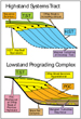
Highstand
In many hydrocarbon exploration
plays, many of the earliest discoveries are found in updip
structural traps, which tend to be dominated by reservoirs of the
HST or highstand sequence set (Figure 16;
Snedden et al., 2002). In some high accommodation basins like West
Africa or Gulf of Mexico, this scales up to the highstand sequence
set
Transgressive
Transgressive
Lowstand
The lowstand The presence of a significant relative sealevel fall causes a major basinward shift in onlap, particularly when shifted seaward of the offlap break. Mid-shelf LST's can also occur (incised valley-fill of Van Wagoner et al., 1990). A common motif on seismic is often toplap/downlap couplets, with toe of clinoform debris wedges or sandstones. These are typically sand rich, although carbonates can also form (the downdip oolite play of the Permian basin).
The vertical succession in a LST
prograding complex is (bottom to top): downlap, progradation, toplap,
aggradation, and floodback (Figure 17).
Earlier models for deepwater settings suggested that there may be
three parts to the LST: the basin-floor
More recent work suggests that
deepwater
The lowstand
One measure of the value of a seismic stratigraphic mapping effort is seen in the ability to address and answer the following key questions: a) Is the petroleum system complete? Is there a critical missing element which will fatally flaw the petroleum system and prevent discoveries in un- or under-explored basin? It is recommended to use the resulting products (cross-sections and maps) to identify source and seals, not just reservoir rocks. For marine source rock mapping, recognition of the large scale, major downlaps (maximum flood) of major continental encroachment cycles is a good starting place (for more detail, see Duval et al., 1998). It is also useful to relate to worldwide eustatic charts and known source bed events. For example, Klemme and Ulmishek (1991) determined that six stratigraphic intervals have provided 90% of the world's discovered original reserves of oil and gas (Silurian-9%, U. Devonian-Tournasian-8%, Pennsylvanian/Lower Permian-8%, Upper Jurassic (25%), Mid-Cretaceous-29%, Oligo-Miocene (12.5%)).
b) Are certain
c) Can the sequence stratigraphic
model built here explain the present distribution of fields and dry
holes? Do the downdip dry-holes define a poorly developed
lowstand d) If the lowstand system tract play corridor can be identified, are downdip prospects located in the major deltaic fairway or marginal to it? Even the world's greatest basinward shift will fail to send sand into a basinal area of interest if no updip deltaic source is present or an appropriate conduit for sand delivery is not in proximity. It is critical to be in the sand "fairway"!! e) Finally, identify possible play types for prospectors: e.g., pre-orogenic HST, if sealed by syn-orogenic shales; LST, if detached and sealed. TST, if sealed by MFS and sourced by 2nd-order TST shales. Summary and Conclusions
This document is meant to be used as
a working guide to seismic stratigraphic interpretation and not to
be used as a strict set of best practices or conceptual basis for
sequence stratigraphic interpretation. It is a gross representation
of regional to lead Much of the methodology described here and in this volume involves interpretation on paper sections and handmade well-ties (paper to paper). Much of any company’s seismic interpretation today is done on a seismic workstation. The use of paper sections is most useful at the early stages of a project, as geoscientists seek to make correlations and establish criteria for identifying horizons. Once a seismic stratigraphic framework is established on some paper sections (hero lines), the geoscientists can make better interpretations and often faster ones, as no delays occur when multiple interpreters cannot agree on correlations, terminology, or ages. Interpretation is then taken to the workstation for efficient and optimized mapping.
AcknowledgementsThe authors appreciate the assistance of Kurt Johnston (EMEC) in preparing seismic examples for this document. ExxonMobil is thanked for permission to publish this document. John Armentrout provided many insights on scale, hierarchy, and source rocks.
References and Further Reading Abreu, V., M. Sullivan, C. Pirmez, and D. Mohrig, 2003, Lateral accretion packages (LAPs): an important reservoir element in deep water sinuous channels: Marine and Petroleum Geology, v. 20, p. 631-648. Abreu, V., P. Teas, Thomas De Brock, Kendall Meyers, Williams Spears, Steve Pierce, and Dag Nummedal, 2002, Reservoir characterization of the South Timbalier 26 Field: The importance of shelf margin deltas as reservoirs in the Gulf of Mexico: AAPG Bulletin, v. 86, p. 212.
Armentrout, J. M., 1991,
Paleontologic constraints on depositional modeling: examples of
integration of biostratigraphy and seismic stratigraphy, Plio-Pleistocene,
Gulf of Mexico, in Seismic Facies and Sedimentary Processes
of Submarine Fans and Turbidite
Armentrout, J.M., S.J. Malecek,
L.B. Fearn, C.E. Sheppard, P.H. Naylor, A.W. Miles, R.J. Demarais,
and R. E. Dunay, 1993, Log motif analysis of Paleogene depositional
Armentrout, J.M., S.J. Malecek, V.R. Mathur, G.L. Neuder, and G.M. Ragan, 1996, Intraslope basin reservoirs deposited by gravity-driven processes: Ship Shoal and Ewing Banks areas, Offshore Louisiana: GCAGS Transactions, v. 46, p. 443-448. Bally, A.W., 1982, Atlas of Seismic Stratigraphy, AAPG Studies in Geology no. 27, 300 p. Brami, T. R., C. Pirmez, C. Archie, S. Heeralal, and K.L. Holman, 2000, Late Pleistocene deep-water stratigraphy and depositional processes, Offshore Trinidad and Tabago: GCS-SEPM, v. 20, p. 104-115. de Graciansky, P. et al., 1998, Mesozoic and Cenozoic Sequence Stratigraphy of European Basins: SEPM Special Publication no. 60, 786 p. Duval, B.C., C. de Janvry, and B. Loiret, 1992, Detailed geoscience reinterpretation of Indonesia's Mahakam delta scores: Oil and Gas Journal, p. 67-72. Duval, B.C., C. Cramez, and P.R. Vail, 1998, Stratigraphic cycles and major marine source rocks, in P. de Graciansky et al., eds., Mesozoic and Cenozoic Sequence Stratigraphy of European Basins: SEPM Special Publication no. 60, p. 43-52. Fulthorpe, C. S., 1991, Geological controls upon seismic sequence resolution: Geology, v. 19, p. 61-65. Garfield T R., 2000, New insight into the three-dimensional architecture of deep-water facies; the product of a multidisciplinary approach. Anonymous, in Brazil 2000; 31st international geological congress; abstract volume. International Geological Congress Abstracts = Congres Geologique International, Resumes. 31; unpag. Greenlee, S.P., 1992, Integrated sequence stratigraphy of Neogene deposits, New Jersey continental shelf and slope: comparison with Exxon model: GSA Bulletin, v. 104, p. 1403-1411.
Haq, B.U., J. Hardenbol, and
P.R. Vail, 1987, Chronology of fluctuating Klemme H.D., and G.F. Ulmishek, 1991, Effective petroleum source rocks of the world; Stratigraphic distribution and controlling depositional factors. AAPG Bulletin, v. 75, p. 1809-1851. Kolla, V., Ph. Bourges, J-M. Urruty, and P. Safa, 2001, Tertiary sinuous channels, offshore Angola, (West Africa) and implications for reservoir architecture: AAPG Bulletin, v. 85, no. 8, p. 1373-1405. Mansor, Y., J.W. Snedden, J.F. Sarg, B.S. Smith, T.H. Kolich, and M.H. Carter, 1999, Pre-drill predictions versus post-drill results: Use of sequence stratigraphic methods in reduction of exploration risk, Sarawak deep-water blocks, Malaysia: Journal of Asian Earth Sciences, v. 17, p. 247-254. McGilvery, T.A., and D.L. Cook, 2003, The influence of local gradients on accommodation space and linked depositional elements across a stepped slope profile, Offshore Brunei, 2003, GCS-SEPM; v. 23, p. 387-420. Mitchum, R.M., Jr. and J.C. Van Wagoner, 1991, High-frequency sequences and their stacking patterns: sequence-stratigraphic evidence of high-frequency eustatic cycles: Sedimentary Geology, v. 70, p. 131-160.
Mitchum, R.M., Jr., J.B.
Sangree, P.R. Vail, and W.W. Wornardt, W. W., 1994, Recognizing
sequences and Posamentier, H.W., G.P. Allen, D.P. James, and M. Tesson, 1992, Forced regressions in a sequence stratigraphic framework: Concepts, examples, and exploration significance: AAPG Bulletin, v. 76, p. 1687-1709. Posamentier, H.A., 2002a, Sequence stratigraphy: Past, present, future and the role of 3D seismic: GCS-SEPM, p. 37-54.
Posamentier, H.W.,
2002b, Ancient shelf ridges-a potentially significant component of
the transgressive Ramsayer, G.R., 1979, Seismic stratigraphy, a fundamental exploration tool: 11th Annual Offshore Technology Conference Proceedings, p. 101-109. Sarg J.F.; and P.J. Lehmann., 1986, Lower-middle Guadalupian facies and stratigraphy, San Andres / Grayburg formations, Permian Basin, Guadalupe Mountains, New Mexico, in George E. Moore and Garner L. Wilde eds., J.F.Sarg, leader, Lower and Middle Guadalupian Facies, Stratigraphy, and Reservoir Geometries; San Andres / Grayburg Formations, Guadalupe Mountains, New Mexico and Texas: Permian basin Section – SEPM Symposium and Guidebook 86-25, p. 1-8. Snedden, J.W., J.F. Sarg, M.J. Clutson, M. Maas, T.E. Okon, M.H. Carter, B.S. Smith, T.H. Kolich, and Md. Y. Mansor, 1996, Using sequence stratigraphic methods in high-supply deltas: examples from the ancient Mahakam and Rajang-Lupar deltas: Proceedings, Indonesian Petroleum Association, 25th Annual Convention, p. 281-295. Snedden, J.W., J.F. Sarg, and Xudong Ying, 2002, Exploration play analysis from a sequence stratigraphic perspective: GCS-SEPM Foundation Research Conference Proceedings, p. 79-97. Thompson, L.B., and J.W. Snedden, 1996, Geology and reservoir description of 1Y1 reservoir, Oso Field, Nigeria, using FMS and dipmeter, in J.A. Pacht, and R.E. Sheriff, eds., Stratigraphic Analysis Utilizing Advanced Geophysical, Wireline, and Borehole Technology for Petroleum Exploration and Production: GCS-SEPM 17th Annual Research Conference, p. 1-11.
Van Wagoner, J.C., et al.,
1988, An overview of the fundamentals of sequence stratigraphy and
key definitions, in C.K. Wilgus et al., eds., Van Wagoner, J.C., et al., 1990, Siliciclastic Sequence Stratigraphy in Well Logs, Cores, and Outcrops: Concepts for High-Resolution of Correlation of Time and Facies: AAPG Methods in Exploration Series no. 7, 55 p. Vail, P.R., R.M. Mitchum, Jr., and R.G. Todd, 1977, Seismic stratigraphy and global changes of sealevel, in Seismic Stratigraphy--Applications to Hydrocarbon Exploration: AAPG Memoir 26, p. 49-212. Vail P R., 1987, Seismic stratigraphy interpretation using sequence stratigraphy; Part 1, Seismic stratigraphy interpretation procedure, in A.W. Bally, ed. Atlas of Seismic Stratigraphy: AAPG Studies in Geology no. 27; v. 1, p. 1-10. |