^GCS-Wave Analysis of Fracture Systems*

By

Bob A. Hardage¹ and Michael V. DeAngelo¹

Search and Discovery Article #40227 (2006)

Posted December 6, 2006

*Adapted from the Geophysical Corner columns, prepared by the authors, in AAPG Explorer, October and November, 2006. Title of column in October, Part 1 here, is the same as that given above; title of column in November, Part 2 here, is “S-Waves and Fractured Reservoirs.” Editor of Geophysical Corner is Bob A. Hardage. Managing Editor of AAPG Explorer is Vern Stefanic; Larry Nation is Communications Director.

¹Bureau of Economic Geology, Austin, Texas ([email protected] )

Most rocks are anisotropic, meaning that their elastic properties are different when measured in different directions. For example, elastic moduli measured perpendicular to bedding differ from elastic moduli measured parallel to bedding – and moduli measured parallel to elongated and aligned grains differ from moduli measured perpendicular to that grain axis. Because elastic moduli affect seismic propagation velocity, seismic wave modes react to rock anisotropy by exhibiting direction-dependent velocity, which in turn creates direction-dependent reflectivity. Repeated tests by numerous people have shown shear (S) waves have greater sensitivity to rock anisotropy than do compressional (P) waves.

Slowly the important role of S-waves for evaluating fracture systems, one of the most common types of rock anisotropy, is moving from the research arena into actual use across fracture prospects. Examples of S-wave technology being used to determine fracture orientation have been published by Gaiser (2004) and Gaiser and Van Dok (2005), for example. It seems timely to introduce one more example

Part1

uGeneral Statement

uFigures 1 & 2

uExample

uConclusion

uComment

uAcknowledgment

uReferences

Part 2 uGeneral statement

uFigure 3

uExample

uLocal difference

uLocal variations

uProof

uAcknowledgment

Part1

uGeneral Statement

uFigures 1 & 2

uExample

uConclusion

uComment

uAcknowledgment

uReferences

Part 2 uGeneral statement

uFigure 3

uExample

uLocal difference

uLocal variations

uProof

uAcknowledgment

Part1

uGeneral Statement

uFigures 1 & 2

uExample

uConclusion

uComment

uAcknowledgment

uReferences

Part 2 uGeneral statement

uFigure 3

uExample

uLocal difference

uLocal variations

uProof

uAcknowledgment

Part1

uGeneral Statement

uFigures 1 & 2

uExample

uConclusion

uComment

uAcknowledgment

uReferences

Part 2 uGeneral statement

uFigure 3

uExample

uLocal difference

uLocal variations

uProof

uAcknowledgment

Part1

uGeneral Statement

uFigures 1 & 2

uExample

uConclusion

uComment

uAcknowledgment

uReferences

Part 2 uGeneral statement

uFigure 3

uExample

uLocal difference

uLocal variations

uProof

uAcknowledgment

Part1

uGeneral Statement

uFigures 1 & 2

uExample

uConclusion

uComment

uAcknowledgment

uReferences

Part 2 uGeneral statement

uFigure 3

uExample

uLocal difference

uLocal variations

uProof

uAcknowledgment

Figures 1 and 2

Figure 1. (Top) Azimuth-dependent PP arrival time and reflectivity from fracture targets A and B. (Bottom) Azimuth-dependent PS arrival time and reflectivity from the same targets. PP reflectivity changes little with azimuth; PS reflectivity varies significantly. PP arrival time changes by 4 ms between azimuths 50° and 140°, whereas PS arrival time changes by 50 ms. Azimuth 50° is the fast-S mode (S1); azimuth 140° is the slow-S mode (S2).

Figure 2. An azimuth-dependent analysis of PS data similar to that shown in Figure 1 was done at each location having a solid circle with an accompanying short arrow. Each arrow shows the local azi muth in which PS reflectivity from interval A was a maximum. The rose diagrams show the fracture azimuths across intervals A and B as interpreted from FMI log data acquired in well C1. The S-wave-based fracture azimuths agree closely with the FMI-based fracture azimuths and allow fracture orientation to be extended across seismic image space.

Return to top.

Example

The prospect considered here involves two fractured carbonate intervals at a depth of a little more than 1800 meters (6000 feet). A small 5.75-km² (2.25-mi²) three-component 3-D seismic survey (3C3D) was acquired to determine whether PP (compressional) and PS (converted-S) data could be used to determine fracture orientation for optimal positioning of a horizontal well.

Figure 1 shows a PP and PS azimuth-dependent data analysis done in a superbin near the center of this survey. At this superbin location, common-azimuth gathers of PP and PS data extending from 0 to 2000-meter offsets were made in narrow, overlapping, 20-degree azimuth corridors. In each of these azimuth corridors, the far-offset traces were excellent quality and were summed to make a single trace showing arrival times and amplitudes of the reflection waveforms from two fracture target intervals A and B. To aid in visually assessing the character of these summed traces, each trace is repeated three times inside its azimuth corridor in the display format used in Figure 1.

Inspection of these azimuth-dependent data shows two important facts:

· PS waves arrive earliest in the azimuth corridor centered 50° east of north (the fast-S mode, S1) and latest in an azimuth direction 140° east of north (the slow-S mode, S2).

· PS waves exhibit a greater variation in arrival times and amplitudes than do their companion PP waves. For example, PP reflectivity from interval A is practically constant in all azimuth directions, whereas PS reflectivity varies significantly with azimuth. Likewise, PP arrival time of event A changes by only 4 ms between azimuth directions 50° and 140°, but PS arrival times change by almost 50 ms, an order of magnitude greater than the variation in PP arrival times.

Azimuth-dependent trace gathers like these were created at many locations across the seismic image space, and the azimuths in which PS reflection amplitudes from fracture intervals A and B were maximum were determined at each analysis location to estimate fracture orientation for each interval. A map of S-wave-based azimuth results for interval A in the vicinity of calibration well C1 is displayed as Figure 2. Shown as rose diagrams on this map are fracture orientations across the two reservoir intervals as interpreted by a service company using Formation Multi- Imaging (FMI) log data acquired in well C1. S-wave estimates of fracture orientations are shown as short arrows at analysis sites near the well. This S-wave-generated map indicates the same fracture orientations interpreted from the FMI log data.

On the basis of this close correspondence between FMI and S-wave estimates of fracture orientation, the operator used S-wave estimates across the total seismic image area to position and orient a horizontal well trending perpendicular to seismic-based fracture orientation. This well found the S-wave estimates of fracture orientation to be accurate across its drilled lateral distance of approximately 1000 meters, and it serves as a good real-world example of the value of S-wave seismic data for evaluating fracture prospects. In this instance, S-wave data provided fracture information that could not be extracted from P-wave data (Figure 1).

Conclusion

We conclude that application of S-wave seismic technology across fracture prospects should be considered by operators when possible.

Post-mortem Comment

This particular horizontal well was not placed in production – even though the well bore intersected a high population of fractures trending perpendicular to the well axis – because too many of the fractures were plugged with cement. That problem sets the stage for a subsequent article, in which we will describe S-wave attributes that can be used to indicate fracture intensity and openness.

Acknowledgment

This research was funded by sponsors of the Exploration Geophysics Laboratory at the Bureau of Economic Geology.

References

Gaiser, James E., 2004, PS-Wave Azimuthal Anisotropy: Benefits for Fractured Reservoir Management: Search and Discovery Article #40120 (2004).

Gaiser, James E., and Richard R. Van Dok, 2005, Converted Shear-Wave Seismic Fracture Characterization Analysis at Pinedale Field, Wyoming: Search and Discovery Article #11024 (2005).

Part 2

S-Waves and Fractured Reservoirs

General Statement

In Part 1, we show that fracture orientation across fractured-reservoir intervals can be determined by azimuth-based analyses of S-wave velocities and reflection amplitudes.

In Part 2, we return to the same 3C3D seismic data used in Part 1 and show how attributes determined from fast-S and slow-S data volumes allow patterns of relative fracture intensity to be determined in a qualitative, not quantitative, manner.

In Figure 1 we show that in a fractured medium, a converted-S wavefield segregates into a fast-S mode and a slow-S mode, and that the azimuth directions in which these fast-S and slow-S modes orient their polarized displacement vectors differ by 90 degrees. Knowing the polarization directions of these two S-wave modes across this particular study area, we processed the 3C3D data to create a fast-S image volume and a slow-S image volume.

(The procedures used to segregate S-wave data into fast-S and slow-S images are exciting topics to geophysicists but are not appropriate to describe in this article.)

Figure 3

Figure 3. (a) Vertical slice from a fast-S volume. (b) Equivalent vertical slice from the companion slow-S volume. A and B are reflections from fractured carbonate reservoirs. Horizons aa through ff are used to measure fast-S and slow-S time thicknesses and amplitude attributes across fractured intervals A and B. SR1 and SR2 define image coordinates where slow-S reflectivity diminishes but fast-S reflectivity does not. T1 and T2 define locations where a fractured interval shows an increase in time thickness in slow-S space that is not observed in fast-S space.

Example

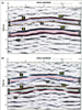
We show here in Figure 3 a vertical slice from the fast-S volume and the corresponding vertical slice from the slow-S volume. The two fractured carbonate intervals A and B are labeled on each display, as well as several horizons interpreted near these two reservoir intervals.

Differences between these fast-S and slow-S images include:

Reflection events A and B arrive approximately 50 ms earlier in the fast-S domain than they do in the slow-S domain.
At certain image coordinates, there are differences between the magnitudes of fast-S and slow-S reflection amplitudes from targets A and B. Two of the more obvious examples are labeled SR1 and SR2.
The fast-S time thicknesses across intervals A and B expand and contract in ways that differ from the expansion and contraction pattern of slow-S time thicknesses.

Some of these relative time-thickness changes are difficult to see by visual inspection of Figure 3, but numerical analyses of the isochron intervals between interpreted horizons show numerous examples of such behavior. Two locations where the time thickness of a reflection wavelet expands more in slow-S image space than in fast-S image space are labeled T1 and T2.

Local Difference: Reflectivity

The units bounding fracture intervals A and B have seismic impedances that are less than the impedances of fracture units A and B. This statement applies to most fractured targets and their bounding units.

Fast-S and slow-S reflectivities across targets A and B are controlled by the magnitude of the differences in impedances across the top and bottom boundaries of A and B. When fracture intensity and fracture openness increase locally, the difference between slow-S and fast-S velocities increases. Fast-S velocity changes little (usually not at all) when fracture intensity increases, but slow-S velocity decreases and becomes closer to the magnitude of the S-wave velocity of its lower-impedance bounding unit. As a result, slow-S reflectivity diminishes, but fast-S reflectivity does not when fracture intensity increases.

To define locations where relative fracture intensity increases, we thus search the fast-S and slow-S volumes to find coordinates where S-wave reflection amplitudes diminish, but fast-S amplitudes change little or not at all. Two image coordinates where this type of reflectivity behavior occurs in Figure 3 are labeled SR1 and SR2. The common interpretation of these differences in fast-S and slow-S reflectivities is that a relative increase in fracture intensity and/or fracture openness occurs at locations SR1 and SR2.

Local Variations: Interval-Time Thickness

When the slow-S interval-time between horizons aa and cc increases (Figure 3b).), two possible explanations are that (1) the thickness of reservoir A has increased or (2) reservoir A has a constant thickness, but slow-S velocity has lowered because of an increase in fracture intensity.

Other arguments may be proposed in different geological settings, but in this case, these two explanations were the most plausible.

· Option 1 can be verified by measuring fast-S interval time between horizons aa and cc (Figure 3a). If the reservoir interval thickens, fast-S interval time should increase.

· If fast-S interval time changes little, or not at all, then option 2 (increased fracture intensity) is accepted as the explanation for the increase in slow-S time thickness.

Two image coordinates where slow-S time thickness increases more than does fast-S time thickness are labeled T1 and T2. Increased fracture intensity is expected at each of these locations.

Prove It!

What we have demonstrated is that comparisons of fast-S and slow-S reflectivities and time thicknesses across fractured intervals allow locations of relative increases in fracture intensity and openness to be identified. These S-wave behaviors indicate only qualitative variations in fracture intensity, not quantitative variations.

Proving the validity of predictions of fracture intensity requires extensive calibration of fast-S and slow-S attributes with reliable fracture maps across prospects. Such investigations are ongoing and will be reported in time. For the present, we show you here the latest logic that seems to allow long-range, seismic definition of relative fracture intensity across multicomponent seismic image space.