![]() Click
to view article in PDF format.
Click
to view article in PDF format.
GCS-Wave Analysis of Fracture Systems*
By
Bob A. Hardage1 and Michael V. DeAngelo1
Search and Discovery Article #40227 (2006)
Posted December 6, 2006
*Adapted from the Geophysical Corner columns, prepared by the authors, in AAPG
Explorer, October and November, 2006. Title of column in October, Part 1 here,
is the same as that given above; title of column in November, Part 2 here, is “S- Waves
Waves and Fractured Reservoirs.”
Editor of Geophysical Corner is Bob A. Hardage. Managing Editor of AAPG Explorer
is Vern Stefanic; Larry Nation is Communications Director.
and Fractured Reservoirs.”
Editor of Geophysical Corner is Bob A. Hardage. Managing Editor of AAPG Explorer
is Vern Stefanic; Larry Nation is Communications Director.
1Bureau of Economic Geology, Austin, Texas ([email protected] )
Most rocks are
anisotropic, meaning that their elastic properties are different when measured
in different directions. For example, elastic moduli measured perpendicular to
bedding differ from elastic moduli measured parallel to bedding – and moduli
measured parallel to elongated and aligned grains differ from moduli measured
perpendicular to that grain axis. Because elastic moduli affect seismic
propagation velocity, seismic wave modes react to rock anisotropy by exhibiting
direction-dependent velocity, which in turn creates direction-dependent
reflectivity. Repeated tests by numerous people have shown shear (S) ![]() waves
waves![]() have
greater sensitivity to rock anisotropy than do compressional (P)
have
greater sensitivity to rock anisotropy than do compressional (P) ![]() waves
waves![]() .
.
Slowly the
important role of S-![]() waves
waves![]() for evaluating fracture systems, one of the most
common types of rock anisotropy, is moving from the research arena into actual
use across fracture prospects. Examples of S-wave technology being used to
determine fracture orientation have been published by Gaiser (2004) and Gaiser
and Van Dok (2005), for example. It seems timely to introduce one more example
for evaluating fracture systems, one of the most
common types of rock anisotropy, is moving from the research arena into actual
use across fracture prospects. Examples of S-wave technology being used to
determine fracture orientation have been published by Gaiser (2004) and Gaiser
and Van Dok (2005), for example. It seems timely to introduce one more example
.
|
Part1uGeneral StatementuFigures 1 & 2uExampleuConclusionuCommentuAcknowledgmentuReferencesPart 2uGeneral statementuFigure 3uExampleuLocal differenceuLocal variationsuProofuAcknowledgment
Part1uGeneral StatementuFigures 1 & 2uExampleuConclusionuCommentuAcknowledgmentuReferencesPart 2uGeneral statementuFigure 3uExampleuLocal differenceuLocal variationsuProofuAcknowledgment
Part1uGeneral StatementuFigures 1 & 2uExampleuConclusionuCommentuAcknowledgmentuReferencesPart 2uGeneral statementuFigure 3uExampleuLocal differenceuLocal variationsuProofuAcknowledgment
Part1uGeneral StatementuFigures 1 & 2uExampleuConclusionuCommentuAcknowledgmentuReferencesPart 2uGeneral statementuFigure 3uExampleuLocal differenceuLocal variationsuProofuAcknowledgment
Part1uGeneral StatementuFigures 1 & 2uExampleuConclusionuCommentuAcknowledgmentuReferencesPart 2uGeneral statementuFigure 3uExampleuLocal differenceuLocal variationsuProofuAcknowledgment
Part1uGeneral StatementuFigures 1 & 2uExampleuConclusionuCommentuAcknowledgmentuReferencesPart 2uGeneral statementuFigure 3uExampleuLocal differenceuLocal variationsuProofuAcknowledgment
|
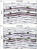
The prospect considered here involves two
fractured carbonate intervals at a depth of a little more than 1800
meters (6000 feet). A small 5.75-km2 (2.25-mi2)
three- Figure 1 shows a PP and PS azimuth-dependent data analysis done in a superbin near the center of this survey. At this superbin location, common-azimuth gathers of PP and PS data extending from 0 to 2000-meter offsets were made in narrow, overlapping, 20-degree azimuth corridors. In each of these azimuth corridors, the far-offset traces were excellent quality and were summed to make a single trace showing arrival times and amplitudes of the reflection waveforms from two fracture target intervals A and B. To aid in visually assessing the character of these summed traces, each trace is repeated three times inside its azimuth corridor in the display format used in Figure 1.
Inspection of these azimuth-dependent data shows two important facts:
·
PS
·
PS
Azimuth-dependent trace gathers like these were created at many locations across the seismic image space, and the azimuths in which PS reflection amplitudes from fracture intervals A and B were maximum were determined at each analysis location to estimate fracture orientation for each interval. A map of S-wave-based azimuth results for interval A in the vicinity of calibration well C1 is displayed as Figure 2. Shown as rose diagrams on this map are fracture orientations across the two reservoir intervals as interpreted by a service company using Formation Multi- Imaging (FMI) log data acquired in well C1. S-wave estimates of fracture orientations are shown as short arrows at analysis sites near the well. This S-wave-generated map indicates the same fracture orientations interpreted from the FMI log data. On the basis of this close correspondence
between FMI and S-wave estimates of fracture orientation, the operator
used S-wave estimates across the total seismic image area to position
and orient a
We conclude that application of S-wave seismic technology across fracture prospects should be considered by operators when possible.
This particular
This research was funded by sponsors of the Exploration Geophysics Laboratory at the Bureau of Economic Geology.
Gaiser, James E., 2004, PS-Wave Azimuthal Anisotropy: Benefits for Fractured Reservoir Management: Search and Discovery Article #40120 (2004). Gaiser, James E., and Richard R. Van Dok, 2005, Converted Shear-Wave Seismic Fracture Characterization Analysis at Pinedale Field, Wyoming: Search and Discovery Article #11024 (2005).
S-
|