![]() Click
to view article in PDF format.
Click
to view article in PDF format.
GCStratal
Slicing Makes Seismic Imaging of  Depositional
 Systems Easier
By
Hongliu Zeng1
Search and Discovery Article #40196 (2006)
Posted June 4, 2006
*Adapted from the Geophysical Corner column, prepared by the author and entitled “Seismic Imaging? Try Stratal Slicing,” in AAPG Explorer, June, 2006. Editor of Geophysical Corner is Bob A. Hardage. Managing Editor of AAPG Explorer is Vern Stefanic; Larry Nation is Communications Director.
1Research scientist, Bureau of Economic Geology, University of Texas, Austin, Texas ([email protected])
Many people today view land surfaces from commercial airplanes or on satellite images and are amazed by the geomorphic forms of river channels, deltas, barrier islands, dune fields, and other features. These views show us modern stratal-time surfaces of exposed landforms.
Three-D seismic technology has now made it possible
to image similar, but much older, geomorphic features and stratal surfaces
preserved in the rock record. Historically, interpreters have analyzed vertical
sections of 3-D seismic volumes line by line and found field-scale (50 meters or
thicker) geologic and ![]() depositional
depositional![]() features. Sometimes, reservoir-scale
(three-10 meters thick) features can be detected in these vertical sections, but
many of these small-scale targets cannot be resolved and interpreted because of
data bandwidth limitations.
features. Sometimes, reservoir-scale
(three-10 meters thick) features can be detected in these vertical sections, but
many of these small-scale targets cannot be resolved and interpreted because of
data bandwidth limitations.
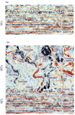
For example, in the vertical view in Figure 1a the seismic facies around the dash line are interpreted to be fluvial deposits, based on the presence of discontinuous, patchy events and frequent lateral changes in amplitudes. Wells drilled through the interval support this interpretation.
However, correlating individual channel-fill sand bodies and marginal facies
(levee, crevasse splay, etc.) on adjacent vertical views is difficult because
these facies elements are thin (three-10 meters) and the seismic resolution
barely resolves the tops and bases of the thickest units. In this particular
section view, it is not possible to decide what ![]() depositional
depositional![]() elements are
represented by the circled features.
elements are
represented by the circled features.
|
uGeneral statementuFigure captionsuSlicesuStratal slicinguAppendix
uGeneral statementuFigure captionsuSlicesuStratal slicinguAppendix
uGeneral statementuFigure captionsuSlicesuStratal slicinguAppendix
|
Time, Horizontal, and Stratal Slices One strategy to
map As a demonstration
of this principle, a stratal slice made by the method described in this
article and then passed through the dash line in
Figure 1a shows high-quality images of fluvial channels, crevasse
splays, floodplain, and a mud plug (Figure 1b).
Although most of these To implement
horizontal-view seismic interpretation, we must pick geologic-time
surfaces (or stratal surfaces) from 3-D seismic volumes so that seismic
attribute maps across these fixed-geologic-time surfaces can be analyzed
in terms of For either horizontal view to be an accurate representation of a stratal surface, one must assume the formation being sliced is flat-lying when time slicing is used (Figure 2a), or that the formation has a sheet-like geometry (Figure 2b) when horizon slicing is used. Many One such method is “stratal slicing” (Figure 2c), or proportional slicing, which divides the variable-thickness vertical interval between two seismic reference events (Figure 2) into a fixed number of uniformly spaced subintervals. If the number of subintervals is 10 and the time thickness between the reference surfaces at points A and B (Figure 2) is 27 ms and 58 ms, respectively, then the thickness of each subinterval at coordinate A is 2.7 ms, and at point B each subinterval is 5.8 ms thick. The interface between each pair of subintervals (the dash lines in Figure 2) approximates a stratal surface. In principle, no major angular unconformities (truncations) or other discordant reflections should occur between the reference events.
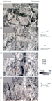
Stratal slices
provide a stratigraphic resolution that cannot be achieved using
vertical sections alone. The data in Figure 3
show a Gulf Coast Pliocene Four stratal slices were taken inside a 30-ms (36-m) interval (Figure 3, S1 through S4). Interpretation of wireline well logs (SP) across the interval shows the sandstones are fluvial in nature. Some of the sandstone units (e.g., a, b and e in Figure 3) are thick (20 to 25 meters) and create amplitude anomalies. Others are thin (10 meters or less) and subtle (c, d and f in Figure 3). In map view, the four stratal slices image four episodes of fluvial deposition (Figure 4, S1 through S4). The fluvial systems on stratal slices S1, S2, and S4 are fully resolved without interference from overlying or underlying units. Stratal slice S3 shows a narrow (35 to 70 meters, or 1 to 2 traces wide), well-developed meandering feature interpreted to be a small coastal plain channel (Figure 4, arrows). Wireline logs indicate this channel-fill sandstone is about four meters thick. Image S3 is only six ms (seven meters) above slice S2 and is contaminated by some interference from the S2 fluvial system. Even so,
The software used to make stratal slices, including necessary reconditioning of seismic data and various attribute applications, was developed by a joint effort of academia and industry, and is available at www.austingeo.com. |