A GIS Approach to the Geology, Production, and Growth of the Barnett Shale Play in Newark East Field, North Texas*

Rick Gonzalez¹

Search and Discovery Article #40147 (2005)

Posted March 27, 2005

*Adapted for online presentation from the Master of Science Project by the author at the University of Texas at Dallas. Mr. Gonzalez’s work (2004) at UT Dallas is posted at http://charlotte.utdallas.edu/mgis/prj_mstrs/2004/Summer/Gonzalez/jegonzalez.htm.

¹University of Texas at Dallas; present residence, Grand Prairie, TX ([email protected]).

Introduction

This paper is a study of the gas-bearing Mississippian Barnett Shale in Newark East Field located northwest of Fort Worth, Texas. Newark East Field straddles most of Wise County, western Denton County, and northwestern Tarrant County. Because it is located near the major urban centers of Dallas and Fort Worth (DFW), it is important to know and understand the developmental state and geology of the most active gas play in the United States. The aim of this study is to gain an insight, by using well data, into the structural geology and its relationship to production patterns. Additionally, the field growth in Newark East is mapped so as to examine its spatial relationship with the surrounding culture and to see the field’s growth in relation to the surrounding urban centers. An analysis of surface lineament trends and their possible relation to the subsurface faulting trends is also discussed.

Figure 1 shows the regional setting in North Texas and the major geologic structures as well as cultural elements that have influenced gas production in Newark East Field. To the northeast the limit is imposed by the Muenster Arch; to the east and south the limits are the urban centers of the DFW area; and to the west the limit until recently had been the Viola Limestone erosional limit (or pinchout) (Figure 2). However, recent improvements in fracturing (stimulation) techniques and drilling methods have begun to allow field expansion west of the edge of the Viola.

The Fort Worth Basin, where the Barnett Shale play is located, encompasses the counties of Clay, Montague, Young, Jack, Wise, Denton, Stephens, Palo Pinto, Parker, Tarrant, Eastland, Erath, Hood, Somervell, Johnson, Comanche, Hamilton, Bosque, Mills, Lampasas, and Coryell in Central and North-central Texas (Figure 1). The aim in this study is to map the formations above and below the Barnett Shale and the growth of the main drilling area where most of the field development has taken place--within Wise, Denton, and Tarrant counties. As of 2003 there have been more than 2800 wells drilled in these counties.

It is worthwhile to mention that the Barnett Shale produces some oil in addition to the gas. This oil is more prevalent in the northern and western parts of Newark East Field, and its production is marginal compared to gas production in the field. Both gas and oil production is mapped in this study.

The Barnett Shale wells require stimulation by fracturing (fracing) in order to obtain commercial (economic) volumes of gas. Early in the existence of the field (1980’s), the stimulation technology did not yet exist for completion of economically successful wells. Through trial and error, Mitchell Energy persisted until they succeeded in developing a technique for fracturing, gel frac, that made the Barnett economically productive. The caveat at the time and up until recently was to keep the fracture stimulation contained within the Barnett. This could be achieved by having the dense Ordovician Viola Limestone below and the dense Pennsylvanian Marble Falls Limestone above. Eventually, in the mid to late 1990’s Mitchell Energy developed a better and less expensive replacement for a gel frac--the slick water frac, which at the time was unconventional for shale stimulation. It became apparent that because of increased interference with neighboring wells water fracs cause a much different fracture pattern than the gel fracs did. Also, wells that were re-stimulated with a water frac produced at even higher rates than when they were initially fraced. Subsequent re-fracturing actually propagated into rock not affected by the first frac, and thereby causing production to increase to rates even higher than obtained after the first stimulation (Bowker, 2002). Once Mitchell perfected the technique and word leaked out to the industry, the play rapidly expanded in the late 1990’s.

The Barnett was deposited over a regional unconformity (Figure 2); the Viola pinches out, or is truncated, below this unconformity just west of Fort Worth and in western Wise County. Because of the missing Viola Limestone, wells drilled on the western part of the main (core) area tend to produce considerable water because the fracture stimulation is not contained extends into the water-bearing Ellenburger Limestone. Until recently drilling had been restricted to east of the Viola erosional limit because it was thought the fracture barriers needed to be present, but drilling and stimulation technology is catching up to the western part of the play. Eventually it will not matter if the fracture barriers above and below the Barnett are present.

This study arose from curiosity about the productive history and geology of the Barnett Shale productive area. Because this is an active and rapidly expanding play, there is the reluctance on the part of some operators to share their data. Most of the work on this play involves geophysical, geochemical data, stimulation techniques, core studies, and thermal maturation history. There have been limited studies related to production and comprehensive geologic maps. Geologic maps submitted to the Texas Railroad Commission are only general in nature; other available maps are broad, regional in nature, encompassing the Fort Worth Basin. The focus of this study is on the Newark East Field area northwest of the DFW Metroplex.

The data obtained for this study are noted, including their format and subsequent manipulation of them. Analysis and methodology applied to the data are explained with the results and discussion.

The stratigraphic units mapped for structural purposes are the Marble Falls Limestone, Barnett Shale, Lower Barnett Shale, and Viola Limestone. A lack of data on the Ellenburger Limestone prevented mapping it. Additionally, lineaments, digitized using DEM data, are compared to subsurface faulting and known studies of fracture orientations to determine if a relationship exists. An isopach map of the gross thickness of the Barnett Shale and three cross-sections have been prepared from well data. ArcScene is used to obtain a 3D model of the subsurface by using the interpolated grids.

Production data are mapped in order to understand where the most productive areas are located, to determine if there are any differences or anomalies in production for different areas of the play, and how the production is related to structure. In this study, Cumulative Gas Production, Cumulative Oil Production, and Practical IP (Initial Potential) are mapped.

Maps were prepared showing the growth of the field since the early 1980’s and how it has expanded near or into some of the surrounding municipalities north and northwest of Fort Worth. The cultural data have been incorporated to illustrate the urban and cultural limits facing operators as field expansion continues. Also, the stake of the main operators in Newark East Field is mapped by showing which wells are operated by whom.

uData

uData

uData

uData

uData

uData

uData

uData

uData

uData

uData

uData

Figure and Table Captions

	Figure 1. Location map of Newark East Field, with regional geologic features.
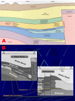	Figure 2. A. Regional cross-section (southwest-northeast), from Parker County to the Muenster Arch, showing generalized stratigraphic and structural relationships. B. Regional cross-sections (east-west and north-south), showing stratigraphic-structural relations in core area of Newark East Field (from Bowker, 2002).
	Figure 3. Cross-section A-A’ (east-west), Newark East Field, showing stratigraphic-structural relationships of Barnett Shale and associated strata.
	Figure 4. Cross-section B-B’ (northwest-southeast), Newark East Field, showing stratigraphic-structural relationships of Barnett Shale and associated strata.
	Figure 5. Cross-section C-C’ (north-south), Newark East Field, showing stratigraphic-structural relationships of Barnett Shale and associated strata.
	Figure 6. Map of wells in Newark East Field categorized according to operator.
	Figure 7. Map of wells that were completed in 1982-1985.
	Figure 8. Map of wells that were completed in 1986-1990.
	Figure 9. Map of wells that were completed in 1991-1995.
	Figure 10. Map of wells that were completed in 1996-1998.
	Figure 11. Map of wells that were completed in 1999-2000.
	Figure 12. Map of wells that were completed in 2001-February, 2004. Click to view sequence of dates of well completions.
	Figure 13. Map showing wells in urban area (DFW Metroplex).
	Figure 14. Structural map, Newark East Field, on top of Marble Falls Limestone.
	Figure 15. Structural map, Newark East Field, on top of Barnett Shale.
	Figure 16. Structural map, Newark East Field, on top of Lower Barnett Shale.
	Figure 17. Structural map, Newark East Field, on top (eroded) of Viola Limestone. Click to view sequence of structural maps.
	Figure 18. Map in 3-D perspective of structure in Newark East Field, with view toward the northwest.
	Figure 19. Isopach map of Barnett Shale (Barnett-Viola interval).
	Figure 20. Map of surface lineaments in the Newark East Field area.
	Figure 21. Map of practical initial potentials (IP) (24-hour flow rate in second month of production).
	Figure 22. Map of cumulative gas produced in Newark East Field.
	Figure 23. Map of cumulative gas produced in part of New East Field, with inset map of well locations.
	Figure 24. Map of cumulative oil produced in Newark East Field.
	Figure 25. Map of cumulative oil produced in part of New East Field, with inset map of well locations.
	Table 1. Orientations of surface lineaments and subsurface faults.
	Table 2. Statistical parameters for orientation of surface lineaments and of subsurface faults.

Return to top.

Previous Work

During the course of this current study, updated information was obtained at the AAPG annual meeting in Dallas (April, 2004) and the Barnett Shale Symposium (June, 2004). Old geologic maps submitted to the Texas Railroad Commission by Mitchell Energy are outdated and general in detail, yet useful; they were used as a check for elements of this study. Additionally, a copy of one of the posters presented at the AAPG meeting, “The Barnett Shale: Not So Simple After All” (Zhao and Givens, 2004), describes the history of the Barnett play since the 1980’s by describing the advancement of stimulation techniques and geologic knowledge. It contains isopach maps of Barnett Shale, formation trends, Fort Worth Basin limits/trends, and major structural elements. Another presentation by Zhao (2004) described the maturation and physical properties of the Barnett shale. “Fractured Shale-gas Systems” (Curtis, 2002) discusses a number of organic shale formations in the United States and focuses on formation lithology, geologic framework, and properties. “Analysis of Natural and Induced Fractures in the Barnett Shale, Mitchell Energy Corporation, T. P. Sims No. 2, Wise County, Texas” (Hill, 1992) characterizes the natural fracture system and the direction of present-day maximum horizontal stress for planning horizontal wells. The findings are meaningful to this current study because lineaments have been mapped in ArcMap. Lineament trends are compared to previous work on Barnett Shale fracturing to determine how these might be related to each other. Additionally, geochemistry studies on the Barnett indicate that the organic-rich Barnett Shale is the primary source rock for oil and gas produced from other Paleozoic age rocks in the Fort Worth Basin (Jarvie et al., 2001; Jarvie and Claxton, 2002). Also, Pollastro et al. (2003) describe the geology, geochemistry, and methodology for assessing undiscovered oil and gas resources using a Total Petroleum System (TPS) method developed by the USGS. The TPS system studied source, reservoir, trap, seals, maturation, and thermal/burial histories. The study eloquently explains structural elements, tectonic history, general stratigraphy, and production history related to the Barnett Shale. An important finding by Pollastro et al., as well as Bowker (2002), is that thermal maturity for hydrocarbons is not related to burial depth, but to heat-flow regimes generated from the Ouachita thrust complex to the east of the play. They state Ouachita thrusting probably influenced hydrocarbon generation in the Fort Worth Basin.

Data

The data collected for this study included well header and production information donated by DrillingInfo.com. Data obtained from their website includes well operator, lease name, lease number, well location, cumulative production, practical IP’s, well status, etc. Because there were more than 2800 wells available from DrillingInfo.com for Newark East, the data had to be downloaded piecemeal. On the website, the easiest way to do this was to query the data by production volumes. Data were downloaded by gas-production-volume ranges to zipped files. The data were provided in comma delimited files. These were subsequently opened in Excel and combined into one spreadsheet named LeaseHeaderData for later use in mapping production data. A total of 2813 wells were obtained. However, not all were used because some of these did not have latitude and longitude; others were repeats. Therefore, the original data had to be edited, and all latitude and longitude values were converted to X-Y values for North Central Texas State Plane Coordinate System 4202, using coordinate conversion software from SeisSoft Company. The X-Y values were added as additional columns to the spreadsheet. North Texas SPCS 4202 was used as the coordinate system for this study. After formatting the data, there were 2384 unique records (wells) as the primary data. Subsequently, the data were imported to the ArcMap geodatabase through Access and saved as the HeaderData table. From ArcMap the wells were mapped directly from the tables by adding these to the view as X-Y event themes.

The Oil Information Library of Fort Worth provided its computer libraries and microfiche well logs. Using a uniform pattern of wells in Newark East Field, tops and other information were keyed into a spreadsheet from IHS Energy’s PI/Dwights database for Texas. Well logs in microfiche form were used to verify the data. Tops were obtained for a total of 884 wells out of the 2384 available in the HeaderData table. These data were imported to the ArcMap geodatabase in a Tops table.

Cultural shape files such as roads, rivers, municipality outlines, county outlines, and freeways were obtained from the 2002 ESRI Data CD’s that come with ArcGIS software. Other shape files, such as the Viola erosional limit, faults, regional structural elements, and lineaments, were generated in ESRI’s ArcCatalog software and digitized in ArcMap. A shape file, named “mask.shp,” was created and used as a mask during raster interpolation of structures. Additionally, DEM and Hillshade grids, from the Texas Natural Resources Information System website, were downloaded for use in the study area.

Also, electric well logs were used to prepare cross-sections across different areas of Newark East Field. These were converted from microfiche to raster TIFF images. They were subsequently cropped in Irfran View software, saved, and imported to GeoPlus’ Petra software. Prior to importing the raster logs, the well locations that were to be used in the cross-sections were imported. Once the TIFFs had been imported to their respective wells, they were depth registered in Petra. This meant assigning depth points to each log in order to calibrate or register its pixel length to the well’s Measured Depth. Also, the tracks were registered for viewing in the Cross Section module. Following this process, three cross-sections were prepared for use in determining and demonstrating structure and formation thicknesses.

Return to top.

Methods

After a personal geodatabase was created in ArcMap, the project’s database in Access, the HeaderData and the Tops spreadsheet, was imported as separate tables. Once this was accomplished, the HeaderData table was added as an X-Y event table in ArcMap. Because this table had each well’s coordinates, it was mapped as an event table. Subsequently, the Tops table was joined in ArcMap to the HeaderData table by the API numbers.

In order to map the tops, a “query by attribute” was performed for each of the formation tops on the joined tables. Once the queries were performed, a table was exported with the selected records into the geodatabase. The same process of querying was performed for the following attributes and saved to the geodatabase: Practical IP, Cumulative Oil, Cumulative Gas, Operator Name, and First Production Date. Thus, the exported tables contained latitude-longitude for each well, along with the queried data for mapping.

For each table for a formation, the preliminary interpolation was done using the Inverse Distance Weighted (IDW) method and the Spatial Analyst with the mask shape file to keep from rasterizing beyond the area where sparse well control is present. The initial set of maps was analyzed for “data busts,” characterized by “bull’s eye” contours, and corrections were made or spurious data deleted. Using the same interpolation method, maps were prepared for Practical IP (24-hour flow rate for the 2^nd month’s production), Cumulative Oil, and Cumulative Gas.

Before finalizing the interpolated structure map for each formation, three cross-sections were made across Newark East Field: Section A-A’, West to East (Figure 3); Section B-B’, Northwest to Southeast (Figure 4); and Section C-C’, North to South (Figure 5). As noted above, the cross-sections allow for verification of the general structure and for the detection of structural and/or stratigraphic changes over the field. Based on the information from cross-sections, the Practical IP map, and well data, faults were digitized on screen as a line shape file. These were used as a barrier to the IDW interpolation technique so that the finalized maps would show the interpreted offset. For all formations, the default IDW technique was used with p-value of 2 and variable search radius with 12 points. The grid size used was 500 feet for all formations. P-values higher than 2 tended to create many bull’s-eye effects on the interpolated maps.

To compensate for the problem due to limited control near faults, especially for the Viola, Marble Falls, and Lower Barnett, some “ghost” wells with tops were created that conform to the anticipated structure in those sparsely controlled areas. This was accomplished by placing the cursor over the desired spot, noting the x-y values, then creating the new ghost well as a new record in the geodatabase table through Access.

The Barnett Shale thickness (isopach) map was constructed by substracting the Barnett Shale interpolated structure from the Viola Limestone interpolated structure, using the map calculator.

Data from the HeaderData table in the geodatabase includes the field Operators. Using these data, the main Operators were mapped in order to show the areas where they operate and have the most acreage. The HeaderData table was queried for Operator. The records of each Operator were saved to a table in the geodatabase. Then, each was loaded as an x-y table event theme in ArcMap and symbolized. Also, Dates of First Production were queried from the HeaderData table to obtain a sense of how the field has expanded since the early 1980’s. These were queried by time intervals: 1982-85, 1986-90, 1991-95, 1996-98, 1999-2000, and 2001-2004. Each interval was saved as a table to the geodatabase and loaded as an x-y table event theme in ArcMap and symbolized.

Finally, an analysis of surface lineaments was performed to determine if the surface expression is related to subsurface fracturing and faulting. Sixty-five surface lineaments were digitized to a shape file on screen by using the DEMs obtained from the Texas Natural Resource Information System. In Excel the data were divided into those that measured from 0 to 89 degrees and those that measured from 90 to 180 degrees (Table 1). Then, the mean for both sets was calculated in Excel.

Results and Discussion

Well Header Information

The analysis of data for Operators in the area gives an idea of where companies are operating and to what extent. In the Barnett Shale trend, Devon is the largest player because of its acquisition of Mitchell Energy wells. The green squares on the map (Figure 6) represent their wells. Most of the production has been from Devon’s wells. The majority of other Operators include Encana, Burlington, Enre, and Chief Energy. Time analysis includes the mapping of First Production Dates for existing wells in Newark East. Figures 7, 8, 9, 10, 11, and 12 show the progression of field expansion since the early 1980’s. From 1982-1985 (Figure 7) twenty one wells were drilled. Throughout each time interval more and more wells are drilled as Michell Energy attempted to extend the field. In 1997 a better stimulation method developed by Mitchell Energy improved well production. Also, the new stimulation method -- water fracing -- was much less expensive than using gel fracs. As noted in Figures 11 and 12, for 1999 to the first part of 2004, the play expanded rapidly as the other operators utilized the new stimulation techniques and as horizontal drilling techniques improved. From the beginning of 2001 to the beginning of 2004, over 1600 wells were first-time producers, representing the highest rate of wells drilled than at any other time interval. This is significant because it shows that drilling activity has been ramping up. As of June, 2004, over 3000 wells had been drilled.

Figure 13 shows the wells and their encroachment on the urban area of the greater DFW Metroplex. What is evident is that well development is not being particularly hindered by culture. Obviously not all areas can be drilled due to limits imposed by urban sprawl and local ordinances. It is estimated that total gas in place for the Barnett Shale is around 26.2 Trillion Cubic Feet (TCF). The Barnett has the potential to be productive under all of Tarrant County and a portion of Dallas County. This is significant because there are urban issues to overcome: Adams (2004) states that “the rapid expansion of drilling into Tarrant County, combined with high rates of population growth, sets the stage for potential conflicts as to land usage, environmental issues, and the rights of mineral owners, pipeline right-of-way issues, visual impact and noise standards, and home-owner-association regulations just to name a few. The Barnett has the potential of becoming one of the largest onshore gas fields in the country.”

Structure

Each formation dips to the northeast (Figures 14, 15, 16, and 17) toward the prominent Muenster Arch, which trends northwest to southeast. Specifically, the Barnett Shale subsea depths range from -5720 to -7628 feet; the highest elevations occur in southeastern Wise County, with elevations decreasing toward the center of Denton County. The cross-sections demonstrate the overall formation dip and faults, represented by blue lines in Figures 14, 15, 16, and 17. Less drilling has occurred in these zones characterized by production of significant volumes of water and little gas. The fractures and faults are thought to be in communication with the water-bearing Ellenburger below the Viola-Simpson rocks. A layered-cake model is illustrated by the 3-D representation of structure (Figure 18). Because the faults are nearly vertical (> 70 degrees--Steward, 2004, personal communication), the structural offsets across a fault can be seen clearly in the 3-D view.

Inspection of Cross-section C-C’ (Figure 5) demonstrates that the Forestburg Limestone, between the Upper Barnett and the Lower Barnett, locally is as much as 200 feet thick; it thins to the south and finally pinches out in the southern part of the field. In Tarrant County the Upper Barnett and Lower Barnett merge into one unit. The Barnett Shale also thins from north to south (Figure 19). It ranges in thickness from about 240 feet in southern Newark East to greater than 1100 feet in the northern area. It is thought that in Mississippian time the shoreline lay to the north relative to Newark East Field, with the limestones, such as the Forestburg, having been deposited in shelf areas and shales deposited in deeper waters.

Return to top.

Lineaments, Faults, and Surface Topography

Average strike of natural fractures is 114^o; average dip is 74^o SW (Hill, 1992). The drilling-induced fractures measured on the FMS log have a mean strike of 54^o, with dip of 81^o NW. Measurements of the very small hydraulic fractures show a mean strike of 60^o and dip of 87^o NW. These results apparently document a change in the stress field from the time the natural fractures formed to the present day. This suggests that “a hydraulic fracture treatment should tend to intersect, rather than parallel, the natural fractures in the Barnett” (Lancaster et al., 1992).

In this study DEM’s were used to map 65 lineaments as line shape files. Figure 20 shows the various lineaments mapped (red lines) over the DEM topography. The subsurface faults have been included on the map to compare with the lineaments. In this study the NE-trending lineaments average 55^o (standard deviation 20, variance 402). SE-trending lineaments average 133^o (standard deviation 34, variance 1172). The subsurface faults, which average 65^o (standard deviation 18, variance 307), may be related to the same stress field; however, the large standard deviation and variance (Table 2) show why this finding is not quite conclusive. On the surface, the SE-trending lineaments would seem to be related to the natural fractures striking 114^o. The NE-trending lineaments would seem to be related to the changed stress field (55^o) noted by Hill (1992). One must keep in mind that Hill’s work was done on one well, the T.P. Sims #2, by studying core fractures and FMS logs at various depths. Also, in Hill’s study, the statistics of the data are not shown; only graphs are presented, and they display a certain degree of variability in the data.

Production Analysis Results

Three interpolated maps were produced from the production data: Practical IP, Cumulative Gas, and Cumulative Oil. Practical IP is the 24-hour rate (Mcd/day) for a well during its second month of production. Figure 21 illustrates where the highest production rates occurred—“away” from the major fault zones (green hues). Closer to the major fault zones, lower rates occur (red hues). Thus, the map clearly shows that the areas of low production rates are due to communication with the Ellenburger Limestone below the Barnett and Viola formations.

Cumulative Gas (Figures 22 and 23) and Cumulative Oil (Figures 24 and 25) maps, respectively, show that most gas and oil production occurs away from the major faulting. It is known that most of the gas produced has come from the core area where Wise, Denton, and Tarrant counties intersect. For the Cumulative Oil map, it is known that crude has been produced in the northern part of the core area. The northern part of the core area is near the edge of the oil-generating window that extends over Clay, Montague, Cooke, and Jack counties (Zhao and Givens, 2004). South of this area is the transition to the gas-generation window, where in Newark East Field the Barnett produces more gas than oil.

Conclusions

As Newark East Field expands, it is encroaching on the DFW area and municipalities. It is evident from the mapping that further growth is being complicated by the urban centers. Producers will have to deal with land-use issues, right-of-way issues, mineral-rights issues, and local ordinances. Expansion of the field appears to be limited to the south and southeast by the population centers.

Mapping and an ArcMap 3-D model show that the Barnett Shale and associated strata dip in the same direction and show a layered-cake-like stratigraphy. The cross-sections aided in determining where the major faulting occurs in Newark East.

Production maps show that the best production is away from the faults. The more heavily faulted areas tend to contain poor gas producers but substantial water production.

There may be some relationship between the surface lineaments and subsurface fracturing and faulting. However, based on the statistics, the relationship is not conclusive. The SE-trending lineaments may be related to the natural fracture orientation of 114^o. The NE-trending lineaments may be related to the induced fracturing of 55^o. Subsurface faults, with the same 55^o orientation, may reflect the same stress field.

References Cited

Adams, G., 2004, Challenges of urban drilling [abs]: Barnett Shale Symposium II, Brookhaven College, Richardson, Texas.

Bowker, K., 2002, Recent developments of the Barnett Shale play, Fort Worth Basin, in Law, B.E., and M. Wilson, eds., Innovative Gas Exploration Concepts Symposium: Rocky Mountain Association of Geologists and Petroleum Technology Transfer Council, October, 2002, Denver, CO, 16 p.

Gonzalez, Rick, 2004, A GIS Approach to the Geology, Production, and Growth of the Barnett Shale Play in Newark East Field: GIS Masters Project: POEC 6386, University of Texas at Dallas (instructor: Instructor: Dr. Ron Brigg) (http://charlotte.utdallas.edu/mgis/prj_mstrs/2004/Summer/Gonzalez/jegonzalez.htm).

Henry, J.D., 1982, Stratigraphy of the Barnett Shale (Mississippian) and associated reefs in the northern Fort Worth basin: Dallas Geological Society paper, 21 p.

Hill, R.E., 1992, Analysis of natural and induced fractures in the Barnett Shale, Mitchell Energy Corporation, T. P. Sims No. 2, Wise County, Texas: Gas Research Institute Report GRI-92/0094, 51 p.

Jarvie, D.M., B.L. Claxton, F. Henk, and J.T. Breyer, 2001, Oil and shale gas from the Barnett Shale, Fort Worth Basin, Texas [abs]: AAPG Annual Meeting, Program and Abstracts, p. A100.

Jarvie, D.M., and B.L. Claxton, 2002, Barnett Shale oil and gas as an analog for other black shales [abs]: AAPG Southwest Section Meeting, Ruidoso, New Mexico.

Jarvie, D. M.,2003, The Barnett shale as a model for unconventional shale gas exploration, presentation for AAPG meeting: Accessed June 2004 at URL http://www.humble-inc.com

Kuuskraa, V.A., G. Koperna, J.W. Schmoker, and J.C Quinn, 1998, Barnett Shale rising star in Fort Worth basin: Oil & Gas Journal, v. 96, no. 21, p. 67-68, 71-76.

Lancaster, D.E. et al, 1992, Reservoir evaluation, completion techniques, and recent results from Barnett Shale development in the Fort Worth basin; Society of Petroleum Engineers, SPE paper 24884, 12 p.

Pollastro, R.M., et al, 2003. Assessing undiscovered resources of the Barnett-Paleozoic total petroleum system, Bend Arch-Fort Worth basin province, Texas: Search and Discovery Article #10034; AAPG Southwest Section Meeting, Fort Worth, Texas. 17 p.

Steward, D.B., 2004, Personal communication: discussion on the Barnett play.

Thomas, J.D., 2003, Integrating synsedimentary tectonics with sequence stratigraphy to understand the development of the Fort Worth basin [abs]: AAPG Southwest Section Meeting, Fort Worth, Texas. 9 p.

Williams, P., 2002, The Barnett Shale: Oil and Gas Investor, v. 22, no 3, p34-45.

Zhao, H., 2004, Thermal maturation and physical properties of Barnett Shale in Fort Worth Basin, North Texas (abs.): AAPG annual convention Dallas (Search and Discovery Article #90026 (http://www.searchanddiscovery.net/documents/abstracts/annual2004/Dallas/Zhao.htm).

Zhao, H., and N. Givens, 2004, The Barnett Shale: not so simple after all: AAPG annual convention Dallas (poster)--Republic Energy Inc. website (http://www.republicenergy.com/Articles/Barnett_Shale/Barnettaspx).

Acknowledgments

I would like to thank the following individuals and/or companies who made this study possible either by donation of their digital data or access to their hard copy files. Their contributions to this project are very much appreciated: The Oil Information Library in Fort Worth and Mr. Roy English for his help while researching at the library; DrillingInfo.com and Charles Hopkins for the production data; Dan B. Steward and Natalie B. Givens at Republic Energy Inc. in Dallas for taking the time to discuss the Barnett Shale and providing material for research; and Bill Harrison, Geoff Ice, Yvette Chovanec, Steve Vonfeldt, Martin Selznick, and Debbie Fierros at Rosewood Resources, Incorporated for their support and encouragement on this project. Also, to my advisor and instructor, Dr. Ron Briggs, University of Texas at Dallas, and to my wife Alicia for “putting up with me” while engrossed in this work.

Return to top.

Search and Discovery
Featured Articles

AAPG Store
Featured Digital Pubs

GIS Map Publishing Program

Online Journal for E&P Geoscientists

Introduction

Previous Work

Data

Search and Discovery
Featured Articles

Archives

AAPG Store
Featured Digital Pubs

GIS Map Publishing Program

Online Journal for E&P Geoscientists

Introduction

Previous Work

Data

Search and DiscoveryFeatured Articles

Archives

AAPG StoreFeatured Digital Pubs

GIS Map Publishing Program

Search and Discovery
Featured Articles

AAPG Store
Featured Digital Pubs