|
Figure Captions
Return to top.
Figure 1
shows a high amplitude reflection characterizing a
Frio reservoir in which gas is trapped
stratigraphically due to a sand pinchout. The
Frio sand, which is about 68 feet thick, is shown in
Figure 2, with the well log synthetic
seismogram tie. Notice that the gas pay has a low velocity compared to
the brine-filled part of the sand at the base. This adds significant
strength to the reflectivity of the sand body, causing it to be seen as
a high amplitude reflection, the classic  bright bright spot. spot.
What cannot be seen is the behavior of
the individual seismic frequencies; i.e., what effect does the
hydrocarbon charge make on the amplitudes of each discrete frequency.
Because the ISA technique allows uncombined reflectivity to be examined,
as no windowing is used during the calculation, the pay reflectivity can
be isolated and studied. This new approach allows one to show the
reflection's response to the hydrocarbon charge at various frequencies
via a "frequency gather," as shown in Figure 3a.The
display shows increasing frequency to the right with the strongest
amplitudes in warm colors.
This is very similar to the familiar
AVO gather -- except where adjacent traces represent the reflection's
response to changing offset in the AVO gather. Here each trace
represents the reflection's amplitude at a single frequency, or
amplitude versus frequency (AVF).
The anomalous response caused by the
pay clearly can be seen as a very high amplitude with a peak frequency
that is shifted toward the high end of the useable bandwidth. When the
process is run on the entire seismic line, single-frequency panels are
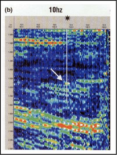
produced, as shown in Figure 3b and 3c. Note
that at 10 Hz, the pay does not exhibit high amplitude, while at 36 Hz,
it is one of the brightest events on the section. The
Frio bright spot on the 36 Hz seismic line in
Figure 3c agrees with the frequency gather shown in
Figure 3a. The pay has relatively little
energy at 10 Hz, but at 36 Hz, it is one of the few remaining events to
have high reflection strength. This is in contrast to the strong events
centered between 2.0 and 2.1 seconds at the wellbore. They have visually
lower frequency and their strongest reflection amplitudes are closer to
10 Hz. When viewed as a frequency panel movie, the changing contrast
becomes very striking. spot on the 36 Hz seismic line in
Figure 3c agrees with the frequency gather shown in
Figure 3a. The pay has relatively little
energy at 10 Hz, but at 36 Hz, it is one of the few remaining events to
have high reflection strength. This is in contrast to the strong events
centered between 2.0 and 2.1 seconds at the wellbore. They have visually
lower frequency and their strongest reflection amplitudes are closer to
10 Hz. When viewed as a frequency panel movie, the changing contrast
becomes very striking.
When the ISA process is applied to
cubes of seismic data, the results are a series of single-frequency
cubes that are loaded onto the workstation and interpreted.
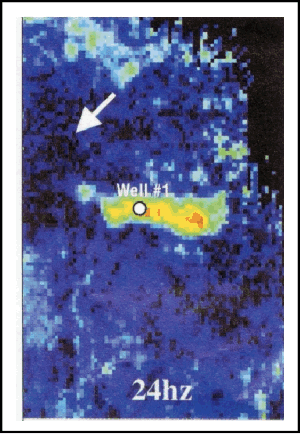
Figure 4 shows four slices from the
frequency cubes on the pay horizon:
-
The first is at 24 Hz, that
frequency which has a minimum amplitude response for the area
surrounding the pay on strike (indicated by the arrows).
-
The second is at 32 Hz, or
near the maximum of the amplitude response at the pay.
-
The third is at 47 Hz,
which shows a minimum in the amplitude spectra of the pay as seen on
the frequency gather at the arrow.
-
The fourth at 58 Hz shows
the reflectivity of the pay close to background.
As Figure 4
shows, the pay is acting completely different than the surrounding sand
when viewed at discrete frequencies. This is even more apparent when all
the frequency maps are viewed as a movie. The pay has a distinctly
different dynamic frequency response than the background because the
hydrocarbons have changed the reflectivity of the reservoir.
To understand the seismic response, let
us examine the detailed reflectivity obtained from well logs.
Figure 5, which shows the modeled response
using sonic and reflectivity logs, explains this difference in dynamic
behavior. The only change between the two curves is that the velocity of
the
Frio pay zone has been replaced by a
brine-filled sand velocity.
The local reflectivity of both cases
has been analyzed for spectral content and is shown in the graph of
amplitude vs. frequency. One can clearly see that the hydrocarbons are
responsible for the high amplitudes at and around 32 Hz and the
associated dimming at 47 Hz. They also are responsible for subtle
changes in reflectivity at other frequencies.
Similarly, the amplitude low at 24 Hz
in the curve with no hydrocarbons can be seen in the maps in the area
surrounding the reservoir.
The sand that produces in this
Frio field is present along strike, pinches out updip, and is not
present downdip. If the observed anomalous reflectivity were due to the
sand thinning, then sequential frequency maps should show a feature
"walking" away from the field; this is not seen. The amplitude maxima of
the reservoir at 32 Hz and the following minima at 47 Hz, plus the
amplitude minima at 24 Hz in the brine-filled area adjacent to the
reservoir observed in the maps, are explained by the spectral modeling.
There could be other geologic
conditions that would cause the reflectivity of this reservoir to more
closely resemble the brine case. A decrease in porosity, for example,
would bring the reservoir velocity closer to that of a brine-filled
sand. In the case of very low porosity, the velocity of the brine and
hydrocarbon-filled sand would be much closer, and the difference in
reflectivity would be much smaller. Thus, the pay would be harder to
discriminate spectrally.
The technique illustrated here will
work best in sands with high porosity and permeability, but it has been
employed successfully in consolidated sands and carbonates in a variety
of depositional environments and depths. Others uses include:
-
The display of attenuation
and low-frequency shadows for direct hydrocarbon indication.
-
The analysis of subtle
thickness or porosity changes, which result in tuning frequency
changes.
Because the input to this process is
simply the migrated data, the better the data quality, the more accurate
the results of this method.
A new type of spectral decomposition
has been shown to be useful as a simple tool to isolate the reflectivity
of hydrocarbons in a
Frio sand reservoir using migrated data.
By viewing frequency maps as a movie,
subtle changes in frequency become dynamically visible. The observed
unique reflectivity of the reservoir due to the presence of hydrocarbons
has been confirmed with its theoretical reflectivity calculated from
well logs. The ISA method of spectral decomposition does not mix the
reflections in time, thus allowing the investigation of reflectivity
from individual seismic events.
This method shows great promise to
become another valuable seismic detection tool in the search for
hydrocarbons.
Return to top.
|
