AAPG GEO 2010 Middle East
Geoscience Conference & Exhibition
Innovative Geoscience Solutions – Meeting Hydrocarbon Demand in Changing Times
March 7-10, 2010 – Manama, Bahrain
Non-Hyperbolic Reflection Tomography for Better Imaging and Interpretation
(1) Nexus Geosciences Inc., Sugar Land, TX.
(2) ConocoPhillips, Houston, TX.
Summary
In this abstract we will demonstrate that the application of non-hyperbolic reflection tomography can produce a 3D subsurface velocity model that is smooth for prestack depth migration and at the same time geological for accurate subsurface pore pressure prediction and lithology interpretation. Our non-hyperbolic reflection tomography workflow is very different from the conventional reflection tomography workflow: no automatic volume picking of residual moveout is used. Instead a set of prestack events are interpreted on prestack seismic ![]() image
image![]() volumes. The prestack events carry detailed moveout information that is more accurate than a single parameter fit to the common
volumes. The prestack events carry detailed moveout information that is more accurate than a single parameter fit to the common ![]() image
image![]()
![]() gathers
gathers![]() . In addition the prestack events carry structure dip information that is needed for accurate 3D ray tracing offset by offset. Examples will be given for both compaction driven and lithology controlled geological environments.
. In addition the prestack events carry structure dip information that is needed for accurate 3D ray tracing offset by offset. Examples will be given for both compaction driven and lithology controlled geological environments.
Introduction
Most production tomography workflow relies on automatic volume picking of residual moveout coefficients, a single parameter description of the moveout variation across offset. Modern seismic acquisition has large source receiver offset (8 kilometer or more). In many minibasin plays the maximum offset is equal to or larger than the basin width. The underlying assumption in most hyperbolic tomography workflow starts to break down: the moveout variation on common ![]() image
image![]() point
point ![]() gathers
gathers![]() can no longer be described by a single parameter, the curvature. Hence the need of non-hyperbolic residual moveout descriptions !
can no longer be described by a single parameter, the curvature. Hence the need of non-hyperbolic residual moveout descriptions !
The quantity “non-hyperbolic residual moveout” is “interpretive” because measuring non-hyperbolic moveouts requires prestack seismic interpretation tools and procedures, which is not available in most desktop applications.
When seismic data is migrated with the correct velocity model, typically the resulting common offset ![]() image
image![]()
![]() gathers
gathers![]() are flat, as opposed to when the migration velocity is not accurate which would result in offset
are flat, as opposed to when the migration velocity is not accurate which would result in offset ![]() gathers
gathers![]() that are not flat. The “non-flatness” depends on the migration model, and is sensitive to other factors such as the dip field. When the model is simple, the offset
that are not flat. The “non-flatness” depends on the migration model, and is sensitive to other factors such as the dip field. When the model is simple, the offset ![]() gathers
gathers![]() analytically follow a hyperbolic curve (Meng & Bleistein, 2001). Otherwise the residual moveout curve would be “non-hyperbolic” — i.e. anything that is not hyperbolic. Differentiating hyperbolic from non-hyperbolic moveouts (Meng et al., 2004) requires a significant change in the tomography workflow, as hyperbolic moveouts can be characterized by one parameter - the curvature - and most reflection tomographic approaches in the literature are based on the single-parameter hyperbolic moveout.
analytically follow a hyperbolic curve (Meng & Bleistein, 2001). Otherwise the residual moveout curve would be “non-hyperbolic” — i.e. anything that is not hyperbolic. Differentiating hyperbolic from non-hyperbolic moveouts (Meng et al., 2004) requires a significant change in the tomography workflow, as hyperbolic moveouts can be characterized by one parameter - the curvature - and most reflection tomographic approaches in the literature are based on the single-parameter hyperbolic moveout.
We describe our non-hyperbolic tomography workflow using one synthetic example and one real data example. The first example is a synthetic example that simulates a compaction driven environment such as the GOM. The second example is a real data example in a lithology driven environment.
It is worthwhile to point out that non-hyperbolic tomography will be more applicable to VTI and TTI migration and velocity model updating, as the migration operators are non-hyperbolic in nature. Using hyperbolic moveout assumption for VTI and TTI tomography is logically inconsistent.
Synthetic Example: GOM Compaction Driven
The synthetic data was provided as a tomographic benchmark test. Only prestack migrated ![]() image
image![]()
![]() gathers
gathers![]() and the migration velocity model were made available during this blind test. The true velocity model used to generate the unmigrated synthetic data was made available only after the completion of the benchmark test.
and the migration velocity model were made available during this blind test. The true velocity model used to generate the unmigrated synthetic data was made available only after the completion of the benchmark test.
Figure 1 shows both the common ![]() image
image![]()
![]() gathers
gathers![]() and our hyperbolic picks (shallow) and non-hyperbolic picks (deep) made on the
and our hyperbolic picks (shallow) and non-hyperbolic picks (deep) made on the ![]() gathers
gathers![]() . Substantial residual moveouts in the whole data volume are visible.
. Substantial residual moveouts in the whole data volume are visible.
A total of 20+ prestack events were picked on the full-volume common ![]() image
image![]()
![]() gathers
gathers![]() . In Figure 1 each color corresponds to an individual prestack event.
. In Figure 1 each color corresponds to an individual prestack event.
After prestack event tracking, the prestack events were demigrated and tomographic inversion was conducted. Fig. 2 (right) shows the final velocity model perturbation from tomographic inversion. Figure 2 (left) shows the true velocity model perturbation that was made available after completion of the benchmark test. As one can see, our tomography has resolved both the low velocity anomaly and the two high velocity anomalies very well: both in the magnitude of velocity correction and in the geometry of the anomalies.
Real Data Example: Lithology Driven Environment
The real data example covers a 1600 km2 area in a lithology-driven environment. The goal of this study was to improve a velocity model starting from existing Kirchhoff ![]() image
image![]()
![]() gathers
gathers![]() . We have employed 3D prestack demigration and remigration (Peng and Sheng, 2009) in the iterative tomography workflow. A third party tomography result was available for comparison. After analyzing the third party’s velocity model, some issues were noted, including: (1) the tomographic result is not usable for lithological intrepretation (Fig. 5, left) because it does not look geological; (2) the starting
. We have employed 3D prestack demigration and remigration (Peng and Sheng, 2009) in the iterative tomography workflow. A third party tomography result was available for comparison. After analyzing the third party’s velocity model, some issues were noted, including: (1) the tomographic result is not usable for lithological intrepretation (Fig. 5, left) because it does not look geological; (2) the starting ![]() image
image![]()
![]() gathers
gathers![]() show large residual errors in the shallow carbonates, while the
show large residual errors in the shallow carbonates, while the ![]() gathers
gathers![]() appeared reasonably flat in the deep target area under a Mass Transport Complex (MTC), a velocity compensating effect over a depth range. These errors in the carbonates introduce significant uncertainty to the interpretation in the deep siliclastical target area (Fig. 4, left).
appeared reasonably flat in the deep target area under a Mass Transport Complex (MTC), a velocity compensating effect over a depth range. These errors in the carbonates introduce significant uncertainty to the interpretation in the deep siliclastical target area (Fig. 4, left).
With access only to the original velocity model and PreSDM ![]() gathers
gathers![]() , we: (1) applied 3D tomography only to the base of carbonates (Tertiary) to correct the large residual errors; (2) demigrated the
, we: (1) applied 3D tomography only to the base of carbonates (Tertiary) to correct the large residual errors; (2) demigrated the ![]() image
image![]()
![]() gathers
gathers![]() using the original velocity model; (3) re-migrated using the new supra-Tertiary velocity model; (4) performed another 3D tomography to the deep target area.
using the original velocity model; (3) re-migrated using the new supra-Tertiary velocity model; (4) performed another 3D tomography to the deep target area.
Figure 3 (left) shows the original multiple-stage tomographic velocity model overlaid on the original stacked ![]() image
image![]() . Figure 3 (right) shows our tomographic velocity model overlaid on the same stacked
. Figure 3 (right) shows our tomographic velocity model overlaid on the same stacked ![]() image
image![]() . Our tomography reveals the high resolution details that are consistent with the lithology. The flatness of the new
. Our tomography reveals the high resolution details that are consistent with the lithology. The flatness of the new ![]() image
image![]()
![]() gathers
gathers![]() (Fig. 4, right) validates our tomography result. This is in contrast to the original tomographically updated model (Fig. 4, left). The lower velocity (in blue color) may be caused by over-pressurized fluids trapped under the carbonates (Fig. 3 right).
(Fig. 4, right) validates our tomography result. This is in contrast to the original tomographically updated model (Fig. 4, left). The lower velocity (in blue color) may be caused by over-pressurized fluids trapped under the carbonates (Fig. 3 right).
Figure 5 shows an interesting area that involves a normal fault in extension setting. The original model was built by a third party using a tomographic workflow (Fig. 5, left). Fig. 5 (right) shows our tomographic results which reveal a higher velocity on the up-throw side (older stratigraphy), and a lower velocity on the down-throw side (younger sedimentary rocks) across the fault. The fault clearly defines a boundary in our velocity model. The new model shows higher velocity at the synclines and lower velocity at the crests, the subtle velocity difference caused possibly by a fluid pressure effect. Supported by both flat ![]() image
image![]()
![]() gathers
gathers![]() and geological consistency, this kind of velocity/impedance inversion may provide invaluable information about fluid migration and caprock sealing effects.
and geological consistency, this kind of velocity/impedance inversion may provide invaluable information about fluid migration and caprock sealing effects.
CONCLUSIONS
We have developed a 3D tomographic velocity updating workflow that uses the non-hyperbolic moveout residues on common ![]() image
image![]()
![]() gathers
gathers![]() . The enabler of this workflow is a prestack seismic interpretation system that permits prestack event tracking on large prestack seismic volumes. A variety of interpretive tools have also been built around the 3D tomography workflow to enable quick and efficient incorporation of geological and geophysical information/knowledge into the process, including QC and editing.
. The enabler of this workflow is a prestack seismic interpretation system that permits prestack event tracking on large prestack seismic volumes. A variety of interpretive tools have also been built around the 3D tomography workflow to enable quick and efficient incorporation of geological and geophysical information/knowledge into the process, including QC and editing.
The tomographic toolkits and the workflow have been tested in GOM salt model building and non-GOM lithology-driven areas. In both cases, the 3D tomographic results proved to be geologically consistent. Our final velocity models also provide higher resolution details in the target areas that can be used for other applications such as pore pressure prediction and fluid migration evaluations.
ACKNOWLEDGEMENTS
The authors sincerely thank BHP Billiton Petroleum USA Inc and its partners for permission to publish these results and the seismic data examples. The synthetic data is provided by ConocoPhillips.
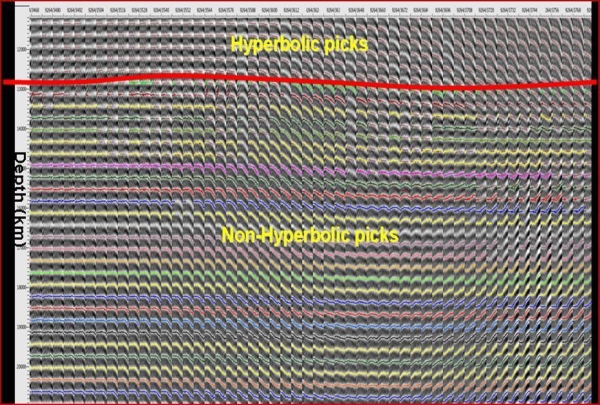 Fig. 1. Non-hyperbolic moveout picks are produced by interpreting horizons on the near offset volume and propagating the seed horizons automatically in offset dimension. They are used as inputs in tomographic updating.
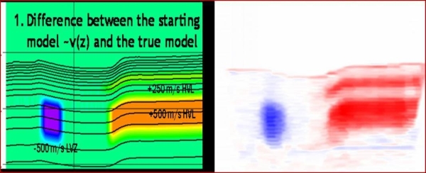 Fig. 2. Synthetic model perturbation (Left) and non-hyperbolic tomographic inversion (Right). Synthetic prestack data is migrated using a velocity model that is a function of V(z) only. Common imaging
 ![]() gathers
gathers![]() and the V(z) model were available for the tomography benchmark test. The true velocity model was disclosed to all participants after submission of the benchmark result. Our non-hyperbolic tomography yields velocity perturbations that are very close to the truth.
and the V(z) model were available for the tomography benchmark test. The true velocity model was disclosed to all participants after submission of the benchmark result. Our non-hyperbolic tomography yields velocity perturbations that are very close to the truth.
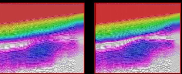 Fig. 3. In this non-GOM example, hard carbonate (limestone) covers a lower velocity mass transport complex (MTC). The left picture shows the original multiple stage tomographic velocity model overlaid on the original stacked
 ![]() image
image![]() ; the right picture shows the higher resolution of the new model overlaid on the same stacked
; the right picture shows the higher resolution of the new model overlaid on the same stacked ![]() image
image![]() .
.
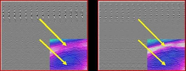 Fig. 4. The left picture shows the
 ![]() gathers
gathers![]() before the interpretive tomography (using the original tomographically updated model) and right shows the
before the interpretive tomography (using the original tomographically updated model) and right shows the ![]() gathers
gathers![]() after the interpretive tomography with some muting applied
after the interpretive tomography with some muting applied
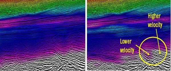 Fig. 5. The left picture shows the original velocity overlaid on the stacked
 ![]() image
image![]() , while the right picture shows the new velocity overlaid on the same stacked
, while the right picture shows the new velocity overlaid on the same stacked ![]() image
image![]() . Our tomography generates a model that shows lower velocity at the down throw and higher velocity at the up-throw side of a normal fault due to expansion. On the left, the new model reveals higher velocity at the synclines and lower velocity at the crests, the velocities on the right are likely caused by fluid pressure effect.
. Our tomography generates a model that shows lower velocity at the down throw and higher velocity at the up-throw side of a normal fault due to expansion. On the left, the new model reveals higher velocity at the synclines and lower velocity at the crests, the velocities on the right are likely caused by fluid pressure effect.