AAPG GEO 2010 Middle East
Geoscience Conference & Exhibition
Innovative Geoscience Solutions – Meeting Hydrocarbon Demand in Changing Times
March 7-10, 2010 – Manama, Bahrain
Depth Velocity Model Optimization Using Beam Migration in a Mediterranean Field Offshore Egypt
(1) PGS Data Processing Middle East, PGS, Cairo, Egypt.
PGS opted to use PGS Beam migration for the depth velocity model building in a Mediterranean field offshore Egypt. The multi-pathing capabilities of PGS Beam migration allow for improved images in proximity to high velocity contrasts or complex geologic regions, while the rapid turn-around time of migrations permits easy confirmation of models. Also the removal of random noise during the dip scanning process provides a good signal to noise gather images suitable for estimating the move-out errors required for tomography updates. These are the characteristics that makes the Beam migration a suitable algorithm to build complex velocity models. In our case study, up to 13 iterations were computed within 12 weeks. During each iteration, most of the time was spent to interpret the results and no time was lost waiting for the migration to complete. The full fold volume of 200 sq.km. was migrated in less than one hour enabling the interpretation of more than one possible velocity model. Once the final velocity model was obtained, the full suite of PSDM algorithms (Beam, Kirchhoff, one way & two way wave equation) could be applied to achieve the best possible image.
Velocity model Building strategy:
The depth velocity model started with a simple DIX converted interval velocity from the available RMS PSTM velocity model. Down to the Messinian, the model was updated using global tomography with two iterations. Top Messinian was structurally updated through interpretation in depth. The Messinian shale/Anhydrite layer was optimized by performing numerous velocity flooding tests to optimize the base of the Messinian. The best flooded model was then subjected to global tomography to optimize the relatively higher velocity channels within the same layer. Five global tomography iterations were run untill the intra- channels as well as the base of the Messinian was giving flat gathers. The base of the Messinian was then interpreted in depth and the velocity model was built using the optimized shale layer with channel velocities determined by the tomography. The image quality for the pre-Messinian deposits were enhanced when compared to the PSTM images (Figures 1 to 4). The variable thickness of the shale layer along with the channels embedded in the same layer had built complex ray paths, that make the RMS velocity not suitable to image the structure below. The advantage of the fast Beam algorithm and the highly defined image was illustrated with which the models were built and verified, at a speed that allows real time “processing and interpretation”. It was then possible for the geologists to perform the interpretation based on the most geological reasonable model.
For the deeper targets between Base Messinian and the top Unconformity we updated the initial model through 6 iterations while performing some lateral smoothing to the model and removing low velocity anomalies. Between the top Unconformity till top Carbonate we used a Vo map at the Unconformity surface with a gradient of 0.2 to reach flat gathers at top Carbonates. Below top Carbonates we have updated the initial model two tomography updates to reach the final model. This sums to a total of about 16 migration production runs to produce the final cube, beside many migration runs to test the different velocity models and updates.
The final velocity model achieved after three months would not be possible using the conventional Kirchhoff migration algorithm. A comparison was made between the Beam algorithm and the Kirchhoff algorithm using the same velocity model to confirm the image quality (Figures 5 & 6). The Beam image was showing lower noise level when compared to the Kirchhoff image.
PGS would like to thank IEOC to grant permission to publish these data examples.
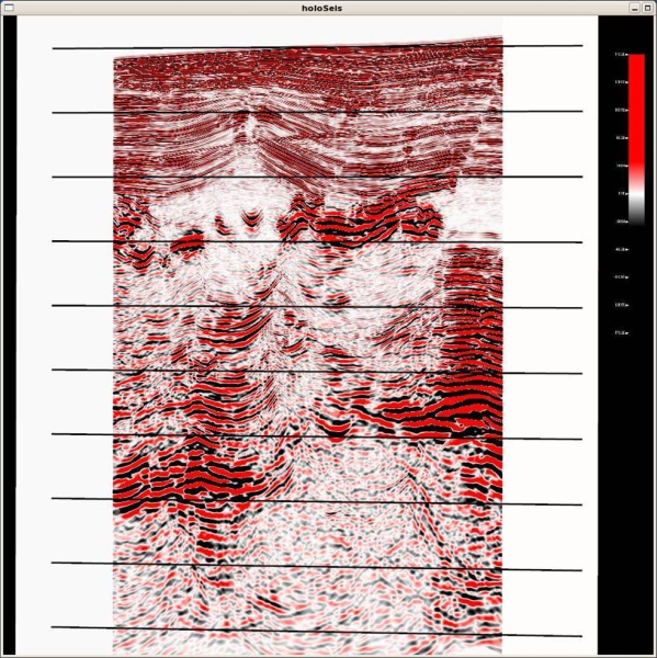
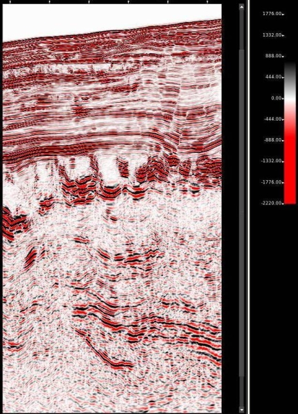 Inline1: PSDM Beam with FInal VM stretch to time
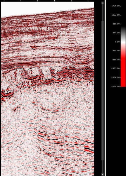
 Inline2: PSDM Beam with final VM stretch to time
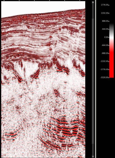
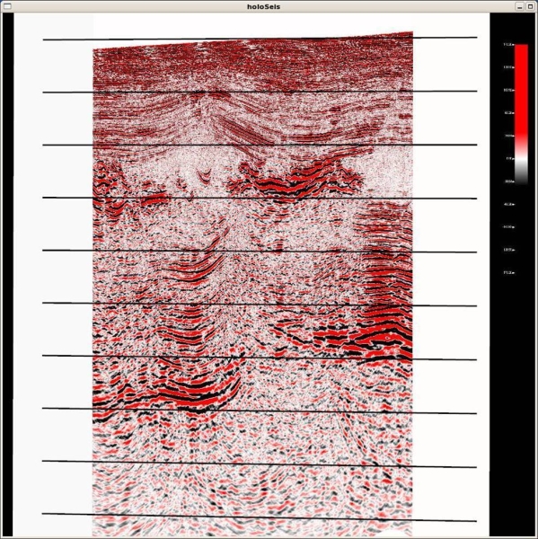
 Inline1: PSTM stack
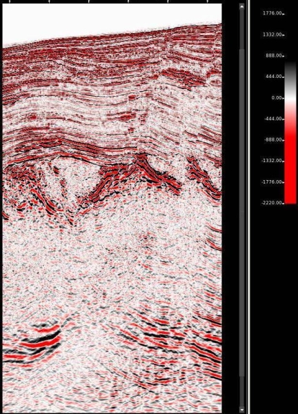 Inline 2: PSTM stack
 PSDM Beam
 PSDM Kirchhoff