Real Time Deep Electrical Images, a Highly Visual Guide for Proactive Geosteering

Roland Chemali¹; Michael Bittar¹; Bronwyn Calleja¹; Amr Lotfy³; Donald Hawkins²

(1) Sperry Drilling, Halliburton, Houston, TX.

(2) Sperry Drilling, Halliburton, East Ahmadi, Kuwait.

(3) Sperry Drilling, Halliburton, Al-Khobar, Saudi Arabia.

Introduction

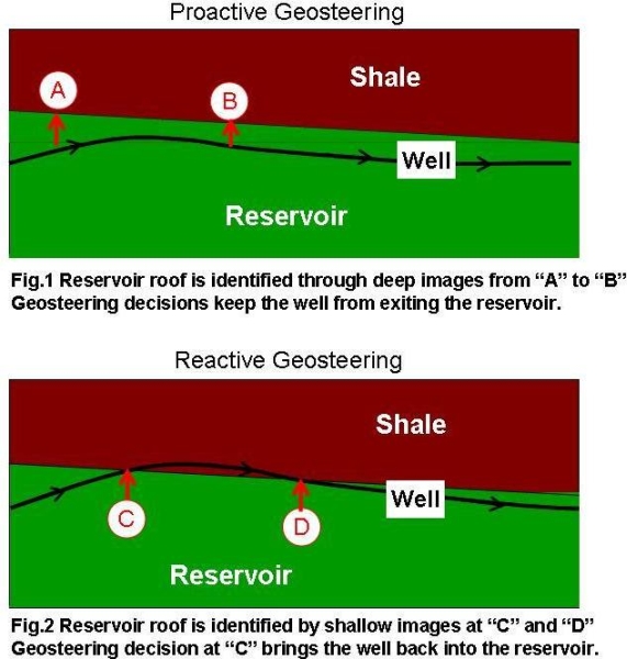
For ideal well placement it is now possible to guide real time decisions with deep electrical images of the surrounding geology. New azimuthal deep resistivity LWD sensors show images of approaching boundaries long before they cross the well path. Clearly the earlier an approaching boundary is detected and mapped in space, the longer the window of opportunity to change the course of the well and to avoid exiting the reservoir. Because the geosteering engineer sees geological events from a distance and makes decisions in advance of crossing reservoir boundaries, the geosteering operation is said to be “proactive”.

Proactive geosteering is best illustrated by comparing it with the more traditional “reactive” geosteering. In reactive geosteering decisions on changes of direction are based on wellbore images or other information available only once a boundary has been crossed. In general reactive geosteering is beneficial in that it detects when a reservoir exit has actually occurred, and points to the most effective direction to re-enter the reservoir. The LWD sensors used in reactive geosteering include micro-electrical images, azimuthal density and azimuthal gamma. The azimuthal data is pulsed to the surface and displayed as unfolded images of the surface of the borehole. The shallow images are analyzed in real time to determine dip and azimuth of encountered geological events and to define the best path to reenter the reservoir if needed.

A conceptual comparison between proactive geosteering and reactive geosteering is illustrated in Fig. 1 and Fig. 2. Observe that in most instances it is preferable to combine both types as they complement each other and back each other up. It will be shown that deep azimuthal resistivity tends to be far-sighted and incapable of mapping a boundary that is very close to the borehole or straddling the borehole. By contrast wellbore images from density, gamma or micro-resistivity can only see boundaries that come within a few inches from the wellbore or cross the wellbore.

Deep Electrical Images from Azimuthal Deep Resistivity

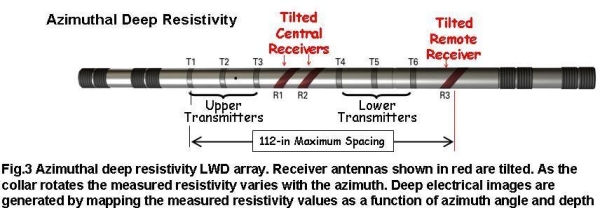
Deep electrical images are generated by a new LWD sensor called azimuthal deep resistivity InSite ADR. A rendering of the coil array is shown in Fig. 3. Detailed description of the sensor and its various functions and outputs is given by Bittar et Al (2007).

The coil array includes various combinations of transmitter-receiver pairs, each operating at two or three frequencies: 125 KHz, 500 KHz and 2 MHz. The azimuthal deep resistivity sensor acquires a total of 36 resistivity logs corresponding to different spacings, to different frequencies and whether they are based on phase or attenuation. Logs measured by longer spacings see generally deeper in the formation. Logs measured at lower frequencies see also deeper in the formation. For each spacing and frequency combination, separate resistivity measurements are derived from phase difference and from attenuation. Attenuation resistivity sees deeper than phase resistivity. These approximate rules of thumbs were developed for the non-azimuthal wave resistivity sensors over the last three decades. They hold also for azimuthal resistivity sensors. Each of the 36 resistivity measurement is acquired every 11.25 deg rotation thus yielding a 32 bin array around the circumference of the borehole.

For ease of interpretation and visualization each azimuthal resistivity data array may be displayed as an image. This has been common practice with all other azimuthally varying measurements including density, micro-resistivity and gamma. The difference in this case is in the region being imaged. Deep resistivity measurements see several feet in the formation away from the well bore. By comparison, micro resistivity images originate within 1 inch from the borehole wall as described in Bittar et al. (2008).

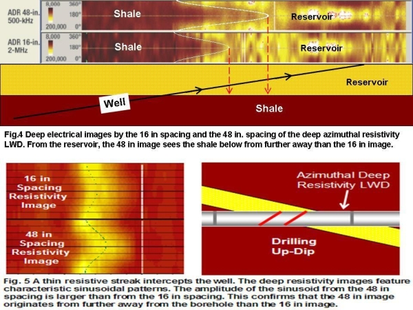
An example of deep electrical images from azimuthal deep resistivity LWD is shown in Fig. 4. This example comes from a horizontal well in the Oseberg field and was reported by Bittar et al. (2008). Observe the two images displayed side by side: one is measured by the 16 inch spacing at 2 MHz and the second by the 48 inch spacing at 500 KHz. From within the higher resistivity sand shown in yellow, the deeper image sees the nearby shale in ochre from further away.

A well known technique for qualitative and quantitative interpretation of borehole images consists of identifying sinusoidal patterns and fitting sinusoids that best approximate those patterns. This technique is based on the simple observation that when a planar event intersects a borehole, the unfolded image of the intersection exhibits an exact sinusoidal shape. The amplitude of the sinusoid is proportional to the tangent of the relative dip angle of the event, and its phase is indicative of the relative azimuth.

This method however is not readily applicable to deep resistivity images like the ones shown in Fig. 5. Those images were reported by Diaz et al. (2009). Although the 48 in. image and the 16 in. image are of the same event, the associated sinusoids have vastly different amplitudes. This observation is consistent with the fact that the two images originate from different regions away from the wellbore. An exact determination of the relative dip of a boundary is still possible by computing the distance between the well and the boundary as the sensor moves, then triangulating for a given finite interval.
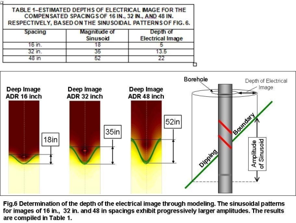
An estimate of the depth of electrical image for azimuthal deep resistivity is obtained by following the same method as for micro-resistivity images (Bittar et al., 2007). A series of computer models are run for a given boundary at 45 degree dip, separating two formations of resistivities 1 and 10, respectively. Fig. 6 shows the computed images for three spacings, 16 in., 32 in. and 48 in. The best fit sinusoids have the following three magnitudes respectively: 18 in., 35 in.,, and 52 in.. Table 1 provides the corresponding depth of the electrical image.

Detecting Boundaries through Bright Spots on the Deep Resistivity Images

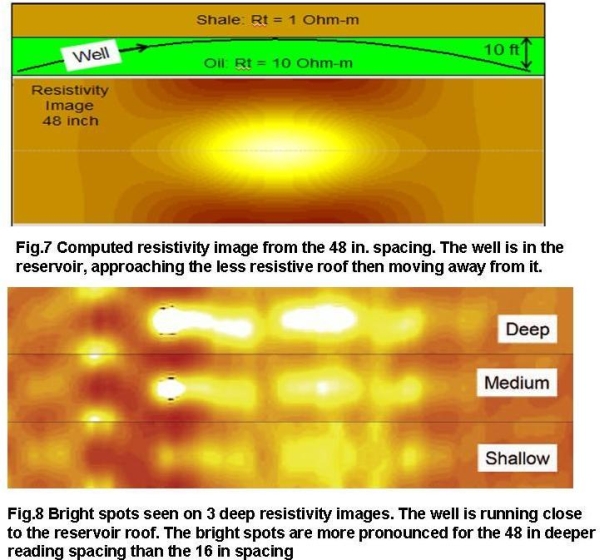
Deep resistivity images exhibit a counter-intuitive phenomenon best described a “bright spots”. In the normal color scheme for resistivity maps, bright yellow or white correspond to high resistivity. For a reason that can be proven only through theoretical modeling, the electrical images of a low resistivity formation yield an abnormally high resistivity reading, often higher than all resistivity values within the region of investigation. As explained by Diaz et Al (2009) and Chemali et Al (2008) the bright spot is an extension of the well-documented horn effect of traditional non-azimuthal wave resistivity described by Anderson et al. (1990).
In the modeled example of Fig 7, the well being drilled in a 10 Ohm-m reservoir approaches the roof of the reservoir at the boundary with an overlaying 1 ohm-m shale. A characteristic bright spot appears on the 48 in. image. The same bright spot is seen on the real log of Fig 8. The image from deeper reading spacing of 48 in. exhibits a stronger bright spot than the image from the shallower reading spacing of 16 in.
The example of Fig. 8 is from a real well, but the images shown are from memory data. It is very seldom that three images are pulsed simultaneously to the surface given the bandwidth limitation in LWD. The well is mostly horizontal. The bright spots seen on the 48 in. image are indicative of the presence of a low resistivity reservoir cap running alongside the well. The intent was to optimally place the well at the highest point in the reservoir but without exiting through the roof. This objective was clearly achieved. For completeness it must be stated that in this instance geosteering was mainly guided by the Geosignal, subject of the next paragraph.

The Geosignal and its Capability to Image Deeper Than Resistivity

For all spacings and for each operating frequency, a 32-bin geosteering signal or geosignal is produced with the ability to detect approaching boundaries from further away than azimuthal resistivity. See Bittar (2002).
The basic geosignal is obtained by measuring phase readings or attenuation readings at the receiver coil at all pairs of opposing angular positions of the collar, then taking their difference. The method is illustrated in Fig. 9 for the case where the opposing angular positions are “up” and “down”. Additional normalization is performed to the geosignal to compensate for and electronic or mechanical drift.

Electrical images obtained from mapping the geosignal generally originate from deeper in the formation than deep azimuthal resistivity images. This advantage of the geosignal images is simply illustrated by computing the geosignal in the simple model of Fig. 7 and mapping it in a similar manner. The results shown in Fig. 10 verify indeed that the geosignal image exhibits an earlier sensitivity to an approaching boundary than the deep resistivity image.

The example of Fig. 11 from a real log confirm that the geosignal images can track a nearby low resistivity formation from further away than resistivity images. Geosignal images however are more difficult to interpret and require prior knowledge of the resistivity sequence in the surrounding geology. From a practical point of view geosteering is performed by integrating the deep resistivity images with the magnitude of the geosignal through dedicated inversion software. See Chemali et al (2008).

Conclusion

Deep electrical images expand the applications of real time images to include the geology surrounding the borehole several feet away from the well path. Deep electrical images include primarily maps of apparent azimuthal resistivity measurements and maps of geosignal measurements. Both types of measurements are acquired by a new type of LWD sensor named azimuthal deep resistivity. Deep electrical images, by virtue of their depth of investigation, anticipate crossing geological boundaries. They forewarn for instance of impending exits from the hydrocarbon zone into non-productive shale or into water bearing intervals. If interpreted properly in real time they contribute significantly to proactive geosteering.
Although sound real time geosteering decisions can be made based on deep electrical images, quantitative interpretation of those images is however not yet possible because the depth from which these images originate within the formation is highly variable. It primarily depends on the resistivity of the medium surrounding the wellbore and the frequency of the particular measurement under consideration. A comprehensive quantitative inversion based on the magnitude of the geosignal is performed to quantify the distance to bed boundary and to derive the apparent dip.

Acknowledgement

The authors wish to thank Halliburton for permission to publish this paper and the oil companies who released their data for advancing the understanding of geosteering with azimuthal deep resistivity

References

Anderson, B., Bonner, S., Luling, M., and Rostal, R. 1990. Response of 2-MHz LWD Resistivity and Wireline Induction Tools in Dipping Beds and Laminated Formations. SPWLA Annual Logging Symposium, Paper A, 24-27 June.
Bittar, M. 2002. Electromagnetic Wave Resistivity Tool Having a Tilted Antenna For Geosteering Within a Desired Payzone. US Patent 6,476,609, Nov 5, 2002.
Bittar, M., Chemali, R., Morys, M. et al. 2008. The Depth-of-Electrical Image a Key Parameter in Accurate Dip Computation and Geosteering. SPWLA Annual Logging Symposium, Paper TT, May 2008.
Bittar, M., Hveding, F., Clegg, N., Johnston, et al. 2008. Maximizing Reservoir Contact in the Oseberg Field Using a New Azimuthal Deep-Reading Technology. Paper SPE 116071 presented at the SPE Annual Technical Conference and Exhibition, Denver, Colorado, USA, 21-24 September.
Bittar, M., Klein, J., Beste, R. et al. 2007. A New Azimuthal Deep-Reading Resistivity Tool for Geosteering and Advanced Formation Evaluation. Paper SPE 109971 presented at the SPE Annual Technical Conference and Exhibition, Anaheim, California, 11-14 November.
Chemali, R., Bittar, M., Hveding, F., Wu, M., Dautel, M. 2008. Integrating Images from Multiple Depths of Investigation and Quantitative Signal Inversion in Real Time for Acurate Well Placement. Paper SPE/IPTC-12547-PP presented at the International Petroleum Technology Conference held in Kuala-Lumpur, Malaysia, 3-5 December.
Diaz, M., Iza, A., Rodas, J., et al. 2009. Successful Geosteering in Ecuador Using the Bright Spot Phenomenon from Deep Resistivity Images. Presented at the SPE Latin American and Caribbean Petroleum Engineering Conference held in Cartagena, Colombia, 31 May-3 June 2009.