![]() Click to view PDF version with images, as originally presented in AAPG
Explorer.
Click to view PDF version with images, as originally presented in AAPG
Explorer.
Synthetic Seismograms: Preparation, Calibration, and Associated Issues
By Thomas E. Ewing*
Search and Discovery Article #40019, (2001)
Adapted for online presentation from articles by same author, entitled “Synthetic Helps Spot the Target” and “Real Answers for Synthetic Issues” in Geophysical Corner, AAPG Explorer, July , 1997, and August, 1997, respectively. Appreciation is expressed to the author and to M. Ray Thomasson, former Chairman of the AAPG Geophysical Integration Committee, and Larry Nation, AAPG Communications Director, for their support of this online version.
*Venus Exploration Inc., San Antonio, Texas ([email protected])
For a prospect with some 2-D or 3-D seismic data, the target level on the seismic data must be identified. With a “bright spot” play, a guess may be made by observation. If there are no wells, it, of course, is a guess. A lot of dry holes result from guessing wrong – even on 3-D seismic data.
What is needed is a way to tie depth-based log data
from key wells into time-based seismic data. In other words, a time-depth chart,
or a ![]() velocity
velocity![]() function (because depth =
function (because depth = ![]() velocity
velocity![]() x time), is required.
x time), is required.
The most common problem--the synthetic does not tie--may be solved through use of other data and preparation of a suite of synthetics from a range of parameters. Reasonable compromises may be made for inadequate log data. Also, added features, such as AVO and modeling routines, are possible.
The process of generating synthetics and calibrating them to real seismic data is as much an art as a science.
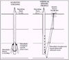 Figure 1.
Configuration of a
Figure 1.
Configuration of a ![]() Velocity
Velocity![]() Survey or VSP.
Survey or VSP.
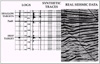 Figure 2. Synthetic Seismograms.
![]() Figure 3.
A 2-D envelope model of a volcanic tuff mound; from Ewing and Caran (1982).
Figure 3.
A 2-D envelope model of a volcanic tuff mound; from Ewing and Caran (1982).
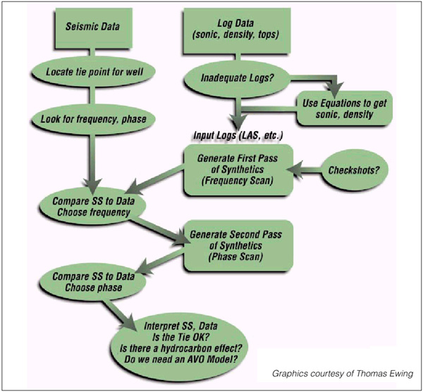 Figure 4.
Flow
chart for tying well-log and seismic data
Figure 4.
Flow
chart for tying well-log and seismic data
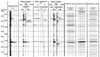 Figure 5:
Comparison of three synthetic seismograms for a deep Yegua well. The left-hand
panels show the comparison of true sonic and density and the logs calculated
using Faust, Gardner and Inverse Gardner (IG). All logs and synthetics are
displayed in time and are corrected by
Figure 5:
Comparison of three synthetic seismograms for a deep Yegua well. The left-hand
panels show the comparison of true sonic and density and the logs calculated
using Faust, Gardner and Inverse Gardner (IG). All logs and synthetics are
displayed in time and are corrected by ![]() velocity
velocity![]() survey (the uncorrected IG-sonic
was considerably too high). The deep, porous gas sandstone depresses density but
not sonic, leading to errors using IG.
survey (the uncorrected IG-sonic
was considerably too high). The deep, porous gas sandstone depresses density but
not sonic, leading to errors using IG.
Ways to Tie Well-Log and Seismic Data
Basics of the Synthetic Seismogram
Compromises: Fabricating Log Data
Ways to Tie Well-Log and Seismic Data
There are three ways to tie well-log and seismic
data.
·
Stacking Velocities derived from seismic
data
These provide the poorest time-depth control. There
are several reasons for this, such as the processors’ need to avoid multiples
and the limited offsets of real seismic data. Stacking velocities are essential
in frontier plays where other data do not exist.
·
![]() Velocity
Velocity![]() Surveys and Vertical Seismic
Profiles (VSP)
Surveys and Vertical Seismic
Profiles (VSP)
VSP give the best ![]() velocity
velocity![]() control. They use a
surface source and geophones downhole (Figure 1). The checkshot uses “first
breaks” (first reception of energy downhole after the shot), while the VSP
analyzes the full sonic waveform over more closely-spaced geophone positions. If
the first breaks are detectable, compression wave (P-wave) time vs. depth is
determined as accurately as possible.
control. They use a
surface source and geophones downhole (Figure 1). The checkshot uses “first
breaks” (first reception of energy downhole after the shot), while the VSP
analyzes the full sonic waveform over more closely-spaced geophone positions. If
the first breaks are detectable, compression wave (P-wave) time vs. depth is
determined as accurately as possible.
·
Synthetic Seismograms derived from well
data
These are a widely useful way to tie seismic time to log depth (Figure 2). Visual matching of seismic and the synthetic can reliably identify the sought-after reflector. Also, the synthetic shows how the detailed waveform and amplitude of the reflectors near the target are generated from the lithology. The interpreter can modify the logs to see what a hydrocarbon reservoir would look like if present. All that is needed is a sonic and density log from a well of interest.
On the minus side, synthetics do not give an
absolute time-depth equivalence; and the synthetic may be a poor match for the
real data. Synthetics may be used with a ![]() velocity
velocity![]() survey to give best possible
time-depth values together with information on reflection character.
survey to give best possible
time-depth values together with information on reflection character.
Basics of the Synthetic Seismogram
A synthetic seismogram is created to simulate
seismic data acquisition in your computer. The unknown physical properties of
the earth beneath a seismic survey are known properties at a wellbore – P-wave
acoustic ![]() velocity
velocity![]() and bulk density. In acquiring seismic data, at the simplest,
a seismic compressional wave (P-wave) is generated with a surface source; the
wave travels at the acoustic
and bulk density. In acquiring seismic data, at the simplest,
a seismic compressional wave (P-wave) is generated with a surface source; the
wave travels at the acoustic ![]() velocity
velocity![]() of the rock, which varies with lithology;
the wave bounces off surfaces across which the impedance – the product of
of the rock, which varies with lithology;
the wave bounces off surfaces across which the impedance – the product of
![]() velocity
velocity![]() and density – varies.
and density – varies.
The strength of the reflection is measured with a
reflection coefficient, which is the difference in impedance over the ![]() sum
sum![]() of the
impedances. The wave then returns to the surface, where geophones detect the
P-
of the
impedances. The wave then returns to the surface, where geophones detect the
P-![]() waves
waves![]() returning vertically. The time from generation of energy to its recovery
at a geophone is the travel time; it depends on the velocities of the units
traversed. The amplitude of the recovered energy is governed by the contrasts in
returning vertically. The time from generation of energy to its recovery
at a geophone is the travel time; it depends on the velocities of the units
traversed. The amplitude of the recovered energy is governed by the contrasts in
![]() velocity
velocity![]() and density across the interfaces.
and density across the interfaces.
All the various geophone groups are recorded; data are processed, and an output section is generated. The interpreter then tries to identify target reflectors in time, analyze the seismic response to geology and fluids, convert time to depth, and drill.
In other words, a source wave is sent through a
![]() velocity
velocity![]() field and a series of reflectors which yield seismic data, or:
field and a series of reflectors which yield seismic data, or:
(Source
Wave)*(![]() Velocity
Velocity![]() Field)**(Reflection Series) = Data
Field)**(Reflection Series) = Data
Geology and hydrocarbons control both velocities
and reflections. The objective is to resolve the reflection series using the
data, knowing the source wave and estimating the ![]() velocity
velocity![]() field:
field:
(Reflection Series)=Data*((Source Wave)*(![]() Velocity
Velocity![]() Field)**) -1
Field)**) -1
This is an “Inverse Problem.” There are direct
and useful ways to do this (called “seismic inversion”), if the phase of the
data is known, and the very low-frequency components of ![]() velocity
velocity![]() and density
that are not captured in seismic data can be added back.
and density
that are not captured in seismic data can be added back.
One of the simplest ways to work the inverse
problem is to take sonic ![]() velocity
velocity![]() and density data from wells, run the seismic
experiment with the sonic-derived
and density data from wells, run the seismic
experiment with the sonic-derived ![]() velocity
velocity![]() field and the sonic- and
density-derived reflection series, assume a source wave similar to the seismic
data, and compare the result to the data.
field and the sonic- and
density-derived reflection series, assume a source wave similar to the seismic
data, and compare the result to the data.
The well data can be varied to match what might exist away from the wellbore--but within the seismic survey. This can be done before the survey is acquired to answer a question such as: “Is a likely target visible?”
A simple synthetic can be made on the back of an envelope, if there are only two or three reflections and great accuracy is not desired. Useful models can be prepared in this way (for example, Ewing and Caran 1982; Figure 3). However, for quantitative work on well logs and for synthetics to match real data, software is needed.
Several good programs exist for synthetic generation – either stand-alone or as a part of a seismic interpretation package. Input log data come from digital files (LAS or LIS), from digitized logs, or from files produced by someone else’s digitization.
Output can be to an inexpensive printer or to a SEG-Y
file that feeds directly into a workstation. One may even hire-out the
process--with a paper log sent out and a synthetic received in return; however,
this process is not interactive and will not result in utilization of the data
to the fullest. The following is a suggested procedure for generating synthetics
and tying them to real seismic data (also see Figure 4):
1. Input sonic and density logs, along with other
log curves as needed for correlation.
2. In the synthetic generation program, run a
Frequency Scan, which calculates traces with a range of frequency filters. The
first trace should include high ![]() frequencies
frequencies![]() , to show the best possible time
resolution of events. The other traces cut off at lower
, to show the best possible time
resolution of events. The other traces cut off at lower ![]() frequencies
frequencies![]() and bracket
the actual frequency of the data at the target depth.
and bracket
the actual frequency of the data at the target depth.
Compare to real data and select the best frequency
filter. If the real data have automatic gain control (AGC), an AGC window can be
applied.
3. Run a Phase Scan. This set of traces should
include zero, 90o, 180o (reversed polarity), 270o
and minimum phase. Compare to real data and select the best phase.
Most airgun or dynamite data are minimum phase;
most vibrator data is either zero or 90o phase.
4. Tie data and synthetic and identify reflectors.
Since log curves do not start at the surface, a few hundred milliseconds of
mistie can be expected.
Calculate the time delay vs. the depth to the top
of the synthetic for a given correlation and determine if the resulting ![]() velocity
velocity![]() seems reasonable--or compare to a nearby
seems reasonable--or compare to a nearby ![]() velocity
velocity![]() survey.
survey.
As the program allows, enter time-depth pairs from a survey and stretch or squeeze the synthetic to fit (this should give a fairly close match to the real data); pay attention to the datums of the synthetic and the seismic.
The most common problem is that the synthetic will
not tie. Variants include:
·
Reflectors seem to come in at the wrong
times.
It cannot be determined which reflector corresponds
to the target. ![]() Velocity
Velocity![]() problems are the main suspect. Synthetics usually need
to be stretched or squeezed to fit data, usually because of an inadequate
measurement of the velocities in the wellbore. This occurs because:
problems are the main suspect. Synthetics usually need
to be stretched or squeezed to fit data, usually because of an inadequate
measurement of the velocities in the wellbore. This occurs because:
1. The hole is washed out; the sonic log fails to
read true formation velocities. There may be cycle skips (which can be removed
editorially). The log “noisiness” may be ![]() different
different![]() for Long-Spaced Sonic vs.
old-fashioned sonic logs.
for Long-Spaced Sonic vs.
old-fashioned sonic logs.
2. The formations are anisotropic. In real seismic,
the energy does not travel purely vertically, but has a horizontal component
which increases at far offsets. If the ![]() velocity
velocity![]() of a formation depends on the
direction of propagation, the rock is anisotropic, the far-offset seismic
of a formation depends on the
direction of propagation, the rock is anisotropic, the far-offset seismic ![]() waves
waves![]() will not travel the same as those in a (vertical) borehole.
will not travel the same as those in a (vertical) borehole.
3. There are dispersion effects. Sonic data in
wells are acquired at kilohertz ![]() frequencies
frequencies![]() , while seismic
, while seismic ![]() waves
waves![]() are usually
less than 120 Hz. If
are usually
less than 120 Hz. If ![]() velocity
velocity![]() varies with frequency, that is dispersion.
varies with frequency, that is dispersion.
The best solution to the problem is to use checkshot information; this is the reason why acquiring it.
Vertical Seismic Profile (VSP) surveys are super-checkshots.
VSPs also provide a direct look at the near-wellbore reflectors at the frequency
band of real seismic. It is recommended that they be used if they are available.
·
The wiggles look ![]() different
different![]() .
.
It is suggested that attempt be made to adjust the frequency and phase content of the wavelet used to create the synthetic. Minimum phase is recommended to match dynamite or airgun data, and zero or 90-degree phase for vibrators. One should observe the final bandpass filters on the header (or conduct a spectral analysis of the data on a workstation).
Synthetics should be compared to VSP data, if
available. Synthetics are an interactive process.
·
There are extra reflections on the real
data.
Real data may contain “multiple energy,” due to
multiple bounces between reflectors within the earth or bounces off the surface
interface. Multiples are usually very weak, because the stacking of modern,
high-fold data discriminates against them. However, if the data are low-fold,
the target is very deep, or the ![]() velocity
velocity![]() profile varies significantly, multiples
may be found in final sections.
profile varies significantly, multiples
may be found in final sections.
Most synthetic programs allow for turning multiples
on or off. Off is usually preferable, but it is simple to compare the two cases.
·
The wiggles are a lot stronger on the
real data than on synthetics, especially at depth.
If the real data are generally strong at depth, the real data may have had an Automatic Gain Control (AGC) filter; the header should be checked. The synthetic seismogram can be run with the same AGC filter.
However, if only one or two reflectors are a lot stronger, this could be an Amplitude vs. Offset (AVO) effect, due to an anomalous amplitude in the far-offset seismic traces.
(Although the Amplitude vs. Offset technology should be reserved for a separate article, it should be noted here that these amplitudes are due to shear-wave generation at an interface by non-orthogonal traces. Because simple synthetic seismograms assume vertical incidence, “zero-offset”, AVO effects are not considered.)
Also, there is usually a considerable difference between the synthetic and the real data due to sampling area. The well-based data will sample a cylinder less than a meter in radius from the well. By contrast, a properly-migrated 3-D seismic trace may sample an area some 10 meters in radius, and the sampling zone in 2-D data could be hundreds of meters in width perpendicular to the line. Sonic and density properties may vary considerably.
VSP data provide major help in this case because it samples the earth at a scale closer to that of real seismic data.
Compromises: Fabricating Log Data
Proper synthetics use sonic and density data – but commonly only one of these, or perhaps only a resistivity curve, is available. The data from these wells may be used in some cases.
Statistical relations exist between ![]() velocity
velocity![]() ,
density, and resistivity. These vary by area and by rock type. The two general
forms are: the Gardner equation, relating density and
,
density, and resistivity. These vary by area and by rock type. The two general
forms are: the Gardner equation, relating density and ![]() velocity
velocity![]() ; and the Faust
equation, relating resistivity and
; and the Faust
equation, relating resistivity and ![]() velocity
velocity![]() . The effects of these techniques are
shown in Figure 5.
. The effects of these techniques are
shown in Figure 5.
If sonic and no density data are available,
synthetics can generally be prepared as usual. The time relationships between
horizons will be accurate because time is based solely on ![]() velocity
velocity![]() ; but the
reflector amplitude will not be completely accurate, for that is based on
impedance (
; but the
reflector amplitude will not be completely accurate, for that is based on
impedance (![]() velocity
velocity![]() times density).
times density).
If density is available, but no sonic, an inverse Gardner relationship should be used. Not all software has this built-in as part of its programs. (Many wells have a density/porosity curve, but not a bulk-density curve. The porosity curve can be used if the mud type is known; the log interpretation manuals should be used.)
If only resistivity is available, Faust’s
equation should be used (Figure 5). Resistivity-generated sonic data usually
need extensive stretching and squeezing to be valid. This requires a good
![]() velocity
velocity![]() function, preferably a trusted
function, preferably a trusted ![]() velocity
velocity![]() survey. In some areas
resistivity will be a poor substitute, but it may be all that is available in
some cases.
survey. In some areas
resistivity will be a poor substitute, but it may be all that is available in
some cases.
For best results, good log suites of wells in a
project area should be used in preparing crossplots of ![]() velocity
velocity![]() , density and
resistivity in order to determine coefficients for the two relationships.
(Neither relationship is very accurate for gas-bearing sandstone, nor are they
useful for evaporites, unless they are identified specifically and are
considered separately.)
, density and
resistivity in order to determine coefficients for the two relationships.
(Neither relationship is very accurate for gas-bearing sandstone, nor are they
useful for evaporites, unless they are identified specifically and are
considered separately.)
First, synthetics can also be generated that
incorporate AVO effects. Determining these effects is very useful, even critical
in many trends for identifying gas-bearing reservoirs or favorable lithologies.
The AVO response of an interface is sensitive to the ratio of compressional-wave
(P-wave) to shear-wave (S-wave) ![]() velocity
velocity![]() . Therefore, in order to generate an AVO
model, the S-wave velocities as well as P-wave velocities need to be known.
. Therefore, in order to generate an AVO
model, the S-wave velocities as well as P-wave velocities need to be known.
The shear velocities come from either a full-waveform sonic log in fast rocks, or a dipole sonic log in slow formations. If no shear information is available, lithology allows an estimate of Vp/Vs; however, this is not very good. If dipole or full-waveform sonic logs are run in any well, the AVO synthetic should be included as normal procedure.
Second, if a series of synthetics in which density
and ![]() velocity
velocity![]() are varied to simulate a geologic or fluid change, a 2-D model is
being created. A set of varying synthetics stitched together along a traverse
approximates a migrated seismic section, but no raypath-dependent effects are
included. Such models are quick, and very useful for understanding the seismic
response to geologic changes. There is software available for this exercise in
many synthetic packages.
are varied to simulate a geologic or fluid change, a 2-D model is
being created. A set of varying synthetics stitched together along a traverse
approximates a migrated seismic section, but no raypath-dependent effects are
included. Such models are quick, and very useful for understanding the seismic
response to geologic changes. There is software available for this exercise in
many synthetic packages.
However, if dips or lateral ![]() velocity
velocity![]() changes are
substantial, or if amplitudes are important, a raytracing algorithm is needed.
These raytracing modelers create a synthetic migrated section but include
shadowing effects due to the bending of raypaths.
changes are
substantial, or if amplitudes are important, a raytracing algorithm is needed.
These raytracing modelers create a synthetic migrated section but include
shadowing effects due to the bending of raypaths.