GC5-D Interpolation Compensates for Poor Sampling*
Daniel Trad¹
Search and Discovery Article #41504 (2014)
Posted December 22, 2014
*Adapted from the Geophysical Corner column, prepared by the authors, in AAPG Explorer, December, 2014. Editor of Geophysical Corner is Satinder Chopra ([email protected]). Managing Editor of AAPG Explorer is Vern Stefanic. AAPG © 2014
¹CGG, Calgary, Canada ([email protected])
Three-D seismic surveys always suffer from poor sampling along at least one spatial dimension – that is why many techniques have been developed over the years to interpolate data, in particular before final migration. Five-dimensional (5-D) interpolation is a wide umbrella covering methods that simultaneously interpolate all space dimensions – and although it is not possible to get the same quality from interpolated traces as the traces recorded in the field, 5-D interpolation has proven to be quite successful. This is reflected in its application in increasingly challenging scenarios with more demanding requirements.
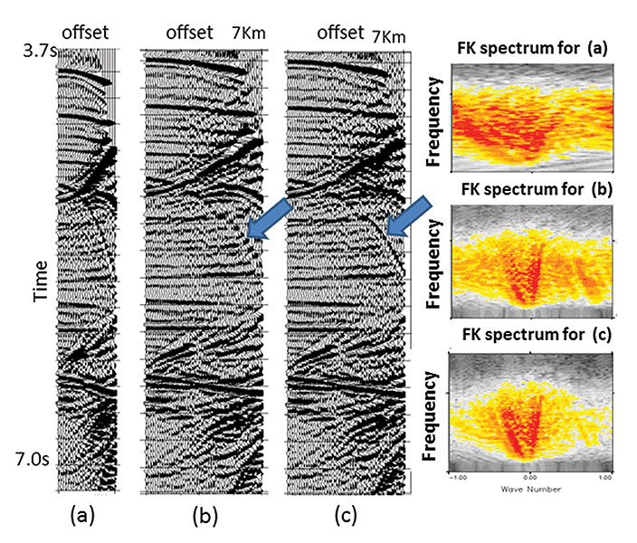
A few years ago interpolation was used to remove sampling artifacts in the stacked image from pre-stack migration; today it is used to improve amplitude analysis in common image gathers and time-lapse studies, which are much more demanding. Although there are many implementations and flavors, the most commonly used algorithms for 5-D interpolation are based on Fourier transforms. They exploit two facts about seismic data:
Interpolation is simply achieved by removing low amplitude energy in the wavenumber domain – with the constraint that the signal has to be well-preserved.
|
♦General statement ♦Figures ♦Interpolators ♦5-D Interpolation ♦Current trends
♦General statement ♦Figures ♦Interpolators ♦5-D Interpolation ♦Current trends
♦General statement ♦Figures ♦Interpolators ♦5-D Interpolation ♦Current trends
♦General statement ♦Figures ♦Interpolators ♦5-D Interpolation ♦Current trends
♦General statement ♦Figures ♦Interpolators ♦5-D Interpolation ♦Current trends |
Differences with Interpolators The breakthrough on 5-D interpolation with respect to previous lower dimensional interpolation algorithms is that information in different dimensions is connected. For example, a gap in the azimuth sampling for one common midpoint ( These restrictions are band limitation and smoothness in the spectrum. Although in practice we can only approximately enforce these constraints, interpolation algorithms often achieve their goal beyond expectations. This is possible because predicted traces do not need to be perfect to help migration algorithms. Although traces created from data interpolation contain only a portion of the information that a real acquired seismic trace would have, this is usually all a migration algorithm will keep after moving and Figure 1 shows a prestack migration result with and without 5-D interpolation. The migration result has clearly improved with interpolation even when the added data do not agree exactly with the unrecorded samples. In many aspects, 5-D interpolation is easier than working on fewer dimensions. For example, this happens when dealing with aliasing, which is the misidentification of high frequency data using lower frequency components. A signal that appears aliased in one dimension may not be aliased in another, and aliased frequencies in multi-dimensions may not overlap in the multidimensional spectra, so it is usually possible to separate them by applying constraints. As a consequence, 5-D algorithms can get around aliasing more easily than lower dimensional interpolators by filtering lower temporal frequencies and carrying information about the localization of wavenumbers to higher temporal frequencies. Furthermore, aliasing is more problematic when spatial samples are located on regular grids – but this never happens in five dimensions. Figure 2 shows a synthetic case from a complex salt environment, which is more difficult than most real scenarios because it has regular sampling and aliasing in all dimensions. In this case the use of standard band limitation plus an artificial sampling perturbation to the interpolation grid helped to interpolate beyond aliasing. In practice, all land surveys have irregularity at least along offset and azimuth directions, and therefore are much easier to interpolate than this example. An area where 5-D interpolation has been seen to be very useful is in merging surveys acquired with different designs and sampling parameters. The mapping of actual spatial sampling to a multidimensional wavenumber domain provides the opportunity for seamless merging of different types of acquisitions. For the same reason it has proven very useful for 4-D studies, although less has been published on this application, mostly for confidentiality issues. However, there are many complications that often compromise the quality of 5-D interpolation results. Its main assumption – that is, sparseness of plane wave events – is not totally realistic. To fulfill it, algorithms work on windows with appropriate overlap and size. Each window typically contains thousands of common midpoints, hundreds of offset bins and several dozens of azimuths. Diffractions are particularly good indicators of interpolation problems, and tend to be the first feature of the data to be affected by poor amplitude preservation. It is crucial to properly preserve diffractions in complex structures and techniques to evaluate the quality of interpolation through proper prediction of diffractions have been proposed. Figure 3 shows a limited-azimuth stack on a complex area before and after interpolation where preservation of diffractions has been essential. Another aspect that often deteriorates results is noise. In principle, random noise does not affect interpolation, because algorithms can only predict coherent energy. Coherent noise, on the other hand, can barely be distinguished from amplitude variations and data complexity, unless strong assumptions are imposed. An interpolator designed to attenuate coherent noise could fail to preserve amplitudes on poorly sampled complex data. Only by introducing additional information and strong assumptions about the data can the algorithm be made robust to noise. Five-D interpolation has become a mature technique in the last decade because of its extensive use for wide-azimuth surveys. There are, however, many unsolved issues and a large effort has been made worldwide to develop new algorithms and solutions. A general trend has been to reduce issues related to binning by using algorithms that can handle exact coordinates. These methods require special care in the use of weights to handle amplitude preservation, but they are becoming easier to use and more flexible. Another trend is to use more information by handling two versions of the data either for noise attenuation or for multicomponent data. Finally, new techniques like least-squares migration attempt the use of basis functions that can capture geological information. Although these techniques can be very expensive from the computational point of view, they have the advantage of including the physics of wave propagation, and therefore may allow geophysicists to go beyond 5-D interpolation. |